【机器学习】使用scikit-learn实现多元线性回归(10min阅读时长)
Multiple Linear Regression(多元线性回归)
之前有一篇简单线性回归的文章,大家感兴趣可以看看。使用scikit-learn实现简单线性回归
Objectives(目标)
看完这篇文章,将会:1.使用scikit-learn实现多元线性回归 2.创建一个模型,训练它,测试它,并使用它
After completing this lab you will be able to:
- Use scikit-learn to implement Multiple Linear Regression
- Create a model, train it, test it and use the model
Table of contents
- Understanding the Data
- Reading the Data in
- Multiple Regression Model
- Prediction
- Practice
Importing Needed packages(导入相关包)
import matplotlib.pyplot as pltimport pandas as pdimport pylab as plimport numpy as np%matplotlib inlineDownloading Data(下载数据)
FuelConsumption(点我下载)
Understanding the Data(理解数据)
FuelConsumption.csv:
我们下载了一个油耗数据集, FuelConsumption.csv,其中包含了加拿大零售新轻型汽车的特定车型油耗等级和估计的二氧化碳排放量。
We have downloaded a fuel consumption dataset, FuelConsumption.csv, which contains model-specific fuel consumption ratings and estimated carbon dioxide emissions for new light-duty vehicles for retail sale in Canada. Dataset source
- MODELYEAR e.g. 2014
- MAKE e.g. Acura
- MODEL e.g. ILX
- VEHICLE CLASS e.g. SUV
- ENGINE SIZE e.g. 4.7
- CYLINDERS e.g 6
- TRANSMISSION e.g. A6
- FUELTYPE e.g. z
- FUEL CONSUMPTION in CITY(L/100 km) e.g. 9.9
- FUEL CONSUMPTION in HWY (L/100 km) e.g. 8.9
- FUEL CONSUMPTION COMB (L/100 km) e.g. 9.2
- CO2 EMISSIONS (g/km) e.g. 182 --> low --> 0
Reading the data in(读取数据)
# df = pd.read_csv("FuelConsumption.csv")df=pd.read_csv("D:\MLwithPython\FuelConsumptionCo2.csv")# take a look at the datasetdf.head()| MODELYEAR | MAKE | MODEL | VEHICLECLASS | ENGINESIZE | CYLINDERS | TRANSMISSION | FUELTYPE | FUELCONSUMPTION_CITY | FUELCONSUMPTION_HWY | FUELCONSUMPTION_COMB | FUELCONSUMPTION_COMB_MPG | CO2EMISSIONS | |
|---|---|---|---|---|---|---|---|---|---|---|---|---|---|
| 0 | 2014 | ACURA | ILX | COMPACT | 2.0 | 4 | AS5 | Z | 9.9 | 6.7 | 8.5 | 33 | 196 |
| 1 | 2014 | ACURA | ILX | COMPACT | 2.4 | 4 | M6 | Z | 11.2 | 7.7 | 9.6 | 29 | 221 |
| 2 | 2014 | ACURA | ILX HYBRID | COMPACT | 1.5 | 4 | AV7 | Z | 6.0 | 5.8 | 5.9 | 48 | 136 |
| 3 | 2014 | ACURA | MDX 4WD | SUV - SMALL | 3.5 | 6 | AS6 | Z | 12.7 | 9.1 | 11.1 | 25 | 255 |
| 4 | 2014 | ACURA | RDX AWD | SUV - SMALL | 3.5 | 6 | AS6 | Z | 12.1 | 8.7 | 10.6 | 27 | 244 |
让我们来选择几个特征去做回归分析
Let’s select some features that we want to use for regression.
cdf = df[['ENGINESIZE','CYLINDERS','FUELCONSUMPTION_CITY','FUELCONSUMPTION_HWY','FUELCONSUMPTION_COMB','CO2EMISSIONS']]cdf.head(9)| ENGINESIZE | CYLINDERS | FUELCONSUMPTION_CITY | FUELCONSUMPTION_HWY | FUELCONSUMPTION_COMB | CO2EMISSIONS | |
|---|---|---|---|---|---|---|
| 0 | 2.0 | 4 | 9.9 | 6.7 | 8.5 | 196 |
| 1 | 2.4 | 4 | 11.2 | 7.7 | 9.6 | 221 |
| 2 | 1.5 | 4 | 6.0 | 5.8 | 5.9 | 136 |
| 3 | 3.5 | 6 | 12.7 | 9.1 | 11.1 | 255 |
| 4 | 3.5 | 6 | 12.1 | 8.7 | 10.6 | 244 |
| 5 | 3.5 | 6 | 11.9 | 7.7 | 10.0 | 230 |
| 6 | 3.5 | 6 | 11.8 | 8.1 | 10.1 | 232 |
| 7 | 3.7 | 6 | 12.8 | 9.0 | 11.1 | 255 |
| 8 | 3.7 | 6 | 13.4 | 9.5 | 11.6 | 267 |
画一下Emission和Engine Size之间的关系
Let’s plot Emission values with respect to Engine size:
plt.scatter(cdf.ENGINESIZE, cdf.CO2EMISSIONS, color='blue')plt.xlabel("Engine size")plt.ylabel("Emission")plt.show()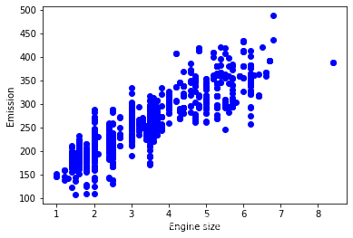
Creating train and test dataset(创建训练集和测试集)
训练/测试分割涉及将数据集分割为互斥的训练集和测试集。 之后,使用训练集进行训练,使用测试集进行测试。
Train/Test Split involves splitting the dataset into training and testing sets that are mutually exclusive. After which, you train with the training set and test with the testing set.
这将对样本外的准确性提供更准确的评估,因为测试数据集不是用于训练模型的数据集的一部分。 因此,它让我们更好地理解我们的模型在新数据上的泛化情况。
This will provide a more accurate evaluation on out-of-sample accuracy because the testing dataset is not part of the dataset that have been used to train the model. Therefore, it gives us a better understanding of how well our model generalizes on new data.
这意味着我们知道测试数据集中每个数据点的结果,这使得它非常适合用于测试! 由于这些数据没有被用来训练模型,所以模型不知道这些数据点的结果。 因此,从本质上讲,这是真正的样本外测试。
This means that we know the outcome of each data point in the testing dataset, making it great to test with! Since this data has not been used to train the model, the model has no knowledge of the outcome of these data points. So, in essence, it is truly an out-of-sample testing.
让我们将数据集分成训练集和测试集。 整个数据集的80%将用于训练,20%用于测试。 我们使用**np.random.rand()**函数创建一个掩码来选择随机行:
Let’s split our dataset into train and test sets. 80% of the entire dataset will be used for training and 20% for testing. We create a mask to select random rows using np.random.rand() function:
msk = np.random.rand(len(df)) < 0.8train = cdf[msk]test = cdf[~msk]Train data distribution(数据的分布)
plt.scatter(train.ENGINESIZE, train.CO2EMISSIONS, color='blue')plt.xlabel("Engine size")plt.ylabel("Emission")plt.show()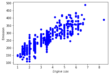
Multiple Regression Model
事实上,影响二氧化碳排放的因素有很多。 当有多个自变量时,这个过程称为多元线性回归。 多元线性回归的一个例子是利用汽车的FUELCONSUMPTION_COMB、EngineSize和Cylinders等特征来预测二氧化碳排放。 这里的好处是多元线性回归模型是简单线性回归模型的扩展。
In reality, there are multiple variables that impact the co2emission. When more than one independent variable is present, the process is called multiple linear regression. An example of multiple linear regression is predicting co2emission using the features FUELCONSUMPTION_COMB, EngineSize and Cylinders of cars. The good thing here is that multiple linear regression model is the extension of the simple linear regression model.
from sklearn import linear_modelregr = linear_model.LinearRegression()x = np.asanyarray(train[['ENGINESIZE','CYLINDERS','FUELCONSUMPTION_COMB']])y = np.asanyarray(train[['CO2EMISSIONS']])regr.fit (x, y)# The coefficientsprint ('Coefficients: ', regr.coef_)Coefficients: [[11.71513251 7.04363114 9.5232153 ]]如前所述,系数和截距是拟合直线的参数。
As mentioned before, Coefficient and Intercept are the parameters of the fitted line.
由于它是一个具有3个参数的多元线性回归模型,参数为超平面的截距和系数,sklearn可以从我们的数据中估计它们。 Scikit-learn使用普通的普通最小二乘法来解决这个问题。
Given that it is a multiple linear regression model with 3 parameters and that the parameters are the intercept and coefficients of the hyperplane, sklearn can estimate them from our data. Scikit-learn uses plain Ordinary Least Squares method to solve this problem.
Ordinary Least Squares (OLS)(最小二乘法–高中就学过)
OLS是一种估计线性回归模型中未知参数的方法。 OLS通过最小化目标因变量与线性函数预测值之差的平方和来选择一组解释变量的线性函数的参数。 换句话说,它试图最小化数据集中所有样本中目标变量(y)和我们的预测输出( y ^ \hat{y} y^)之间的平方误差(SSE)或均方误差(MSE)的总和。
OLS is a method for estimating the unknown parameters in a linear regression model. OLS chooses the parameters of a linear function of a set of explanatory variables by minimizing the sum of the squares of the differences between the target dependent variable and those predicted by the linear function. In other words, it tries to minimizes the sum of squared errors (SSE) or mean squared error (MSE) between the target variable (y) and our predicted output ( y ^ \hat{y} y^) over all samples in the dataset.
OLS可以通过以下方法找到最佳参数:
OLS can find the best parameters using of the following methods:
- Solving the model parameters analytically using closed-form equations
- Using an optimization algorithm (Gradient Descent, Stochastic Gradient Descent, Newton’s Method, etc.)
Prediction(预测)
y_hat= regr.predict(test[['ENGINESIZE','CYLINDERS','FUELCONSUMPTION_COMB']])x = np.asanyarray(test[['ENGINESIZE','CYLINDERS','FUELCONSUMPTION_COMB']])y = np.asanyarray(test[['CO2EMISSIONS']])print("Residual sum of squares: %.2f" % np.mean((y_hat - y) ** 2))# Explained variance score: 1 is perfect predictionprint('Variance score: %.2f' % regr.score(x, y))Residual sum of squares: 538.19Variance score: 0.85Explained variance regression score:
Let y ^ \hat{y} y^ be the estimated target output, y the corresponding (correct) target output, and Var be the Variance (the square of the standard deviation). Then the explained variance is estimated as follows:
explainedVariance ( y , y ^ ) = 1 − Var y − y ^ Vary \texttt{explainedVariance}(y, \hat{y}) = 1 - \frac{Var{ y - \hat{y}}}{Var{y}} explainedVariance(y,y^)=1−VaryVary−y^
The best possible score is 1.0, the lower values are worse.(越接近于1越好)
Practice(练习)
Try to use a multiple linear regression with the same dataset, but this time use FUELCONSUMPTION_CITY and FUELCONSUMPTION_HWY instead of FUELCONSUMPTION_COMB. Does it result in better accuracy?
# write your code hereregr = linear_model.LinearRegression()x = np.asanyarray(train[['ENGINESIZE','CYLINDERS','FUELCONSUMPTION_CITY','FUELCONSUMPTION_HWY']])y = np.asanyarray(train[['CO2EMISSIONS']])regr.fit (x, y)# The coefficientsprint ('Coefficients: ', regr.coef_)# 预测y_hat= regr.predict(test[['ENGINESIZE','CYLINDERS','FUELCONSUMPTION_CITY','FUELCONSUMPTION_HWY']])x = np.asanyarray(test[['ENGINESIZE','CYLINDERS','FUELCONSUMPTION_CITY','FUELCONSUMPTION_HWY']])y = np.asanyarray(test[['CO2EMISSIONS']])print("Residual sum of squares: %.2f" % np.mean((y_hat - y) ** 2))# Explained variance score: 1 is perfect predictionprint('Variance score: %.2f' % regr.score(x, y))Coefficients: [[11.77637455 6.7350317 5.99648967 3.30209632]]Residual sum of squares: 537.85Variance score: 0.85 开发者涨薪指南
  48位大咖的思考法则、工作方式、逻辑体系