统计学习导论之R语言应用(四):分类算法R语言代码实战
统计学习导论之R语言应用(ISLR)
参考资料:
The Elements of Statistical Learning
An Introduction to Statistical Learning
统计学习导论(二):统计学习概述
统计学习导论(三):线性回归
统计学习导论(四):分类
统计学习导论之R语言应用(二):R语言基础
统计学习导论之R语言应用(三):线性回归R语言代码实战
统计学习导论之R语言应用(四):分类算法R语言代码实战
文章目录
- 统计学习导论之R语言应用(ISLR)
- 4.分类
-
- 4.1 探索Smarket数据
- 4.2 logistic regression
- 4.3线性判别分析(LDA)
- 4.4 二次判别分析
- 4.5 朴素贝叶斯
- 4.6 KNN
- 4.7 泊松回归
4.分类
首先我们探索一下Smarkt数据的数字特征。该数据集包括从2001年初到2005年底,标准普尔500指数1250天内的收益率百分比。对于每个交易日,我们都记录了前五个交易日(lagone至lagfive)的回报率百分比。我们还记录了volume(前一天交易的股票数量,以十亿计)、Today(相关日期的回报百分比)和direction(当天市场是上涨还是下跌)。我们的目标是使用其他特征预测是上升还是下降(定性响应)。显然这是一个二分类问题。
4.1 探索Smarket数据
# 导入相关库和数据library(ISLR2)names(Smarket)- 'Year'
- 'Lag1'
- 'Lag2'
- 'Lag3'
- 'Lag4'
- 'Lag5'
- 'Volume'
- 'Today'
- 'Direction'
#查看数据的纬度dim(Smarket)- 1250
- 9
#描述性统计summary(Smarket) Year Lag1 Lag2 Lag3 Min. :2001 Min. :-4.922000 Min. :-4.922000 Min. :-4.922000 1st Qu.:2002 1st Qu.:-0.639500 1st Qu.:-0.639500 1st Qu.:-0.640000 Median :2003 Median : 0.039000 Median : 0.039000 Median : 0.038500 Mean :2003 Mean : 0.003834 Mean : 0.003919 Mean : 0.001716 3rd Qu.:2004 3rd Qu.: 0.596750 3rd Qu.: 0.596750 3rd Qu.: 0.596750 Max. :2005 Max. : 5.733000 Max. : 5.733000 Max. : 5.733000 Lag4 Lag5Volume Today Min. :-4.922000 Min. :-4.92200 Min. :0.3561 Min. :-4.922000 1st Qu.:-0.640000 1st Qu.:-0.64000 1st Qu.:1.2574 1st Qu.:-0.639500 Median : 0.038500 Median : 0.03850 Median :1.4229 Median : 0.038500 Mean : 0.001636 Mean : 0.00561 Mean :1.4783 Mean : 0.003138 3rd Qu.: 0.596750 3rd Qu.: 0.59700 3rd Qu.:1.6417 3rd Qu.: 0.596750 Max. : 5.733000 Max. : 5.73300 Max. :3.1525 Max. : 5.733000 Direction Down:602 Up :648 #变量散点图pairs(Smarket)
cor()函数生成一个矩阵,其中包含数据集中预测变量之间的所有成对相关性。下面的第一个命令给出错误消息,因为direction变量是定性的。
cor(Smarket)Error in cor(Smarket): 'x' must be numericTraceback:1. cor(Smarket)2. stop("'x' must be numeric")cor(Smarket[, -9]) #负号表示去除该列| Year | Lag1 | Lag2 | Lag3 | Lag4 | Lag5 | Volume | Today | |
|---|---|---|---|---|---|---|---|---|
| Year | 1.00000000 | 0.029699649 | 0.030596422 | 0.033194581 | 0.035688718 | 0.029787995 | 0.53900647 | 0.030095229 |
| Lag1 | 0.02969965 | 1.000000000 | -0.026294328 | -0.010803402 | -0.002985911 | -0.005674606 | 0.04090991 | -0.026155045 |
| Lag2 | 0.03059642 | -0.026294328 | 1.000000000 | -0.025896670 | -0.010853533 | -0.003557949 | -0.04338321 | -0.010250033 |
| Lag3 | 0.03319458 | -0.010803402 | -0.025896670 | 1.000000000 | -0.024051036 | -0.018808338 | -0.04182369 | -0.002447647 |
| Lag4 | 0.03568872 | -0.002985911 | -0.010853533 | -0.024051036 | 1.000000000 | -0.027083641 | -0.04841425 | -0.006899527 |
| Lag5 | 0.02978799 | -0.005674606 | -0.003557949 | -0.018808338 | -0.027083641 | 1.000000000 | -0.02200231 | -0.034860083 |
| Volume | 0.53900647 | 0.040909908 | -0.043383215 | -0.041823686 | -0.048414246 | -0.022002315 | 1.00000000 | 0.014591823 |
| Today | 0.03009523 | -0.026155045 | -0.010250033 | -0.002447647 | -0.006899527 | -0.034860083 | 0.01459182 | 1.000000000 |
正如大家所预料的,滞后变量和今天的回报之间的相关性接近于零。换句话说,今天的回报和前几天的回报之间似乎没有什么相关性。唯一实质性的相关性是年份和数量之间的相关性。通过绘制按时间顺序排列的数据,我们可以看到数据量随着时间的推移而增加。换句话说,从2001年到2005年,平均每天交易的股票数量有所增加。
#绘制交易散点图,如下。attach(Smarket)plot(Volume)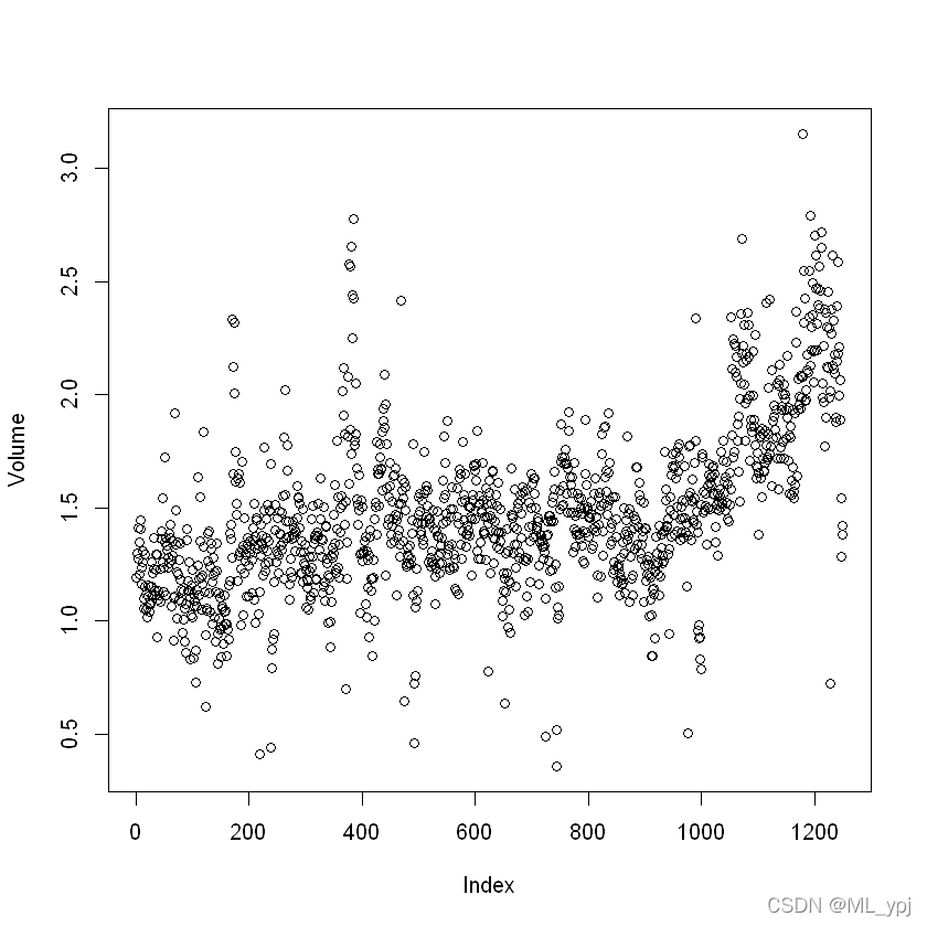
4.2 logistic regression
接下来,我们将拟合一个逻辑回归模型,使用lagone到lagfive和volume预测方向。glm()函数可用于拟合多种类型的广义线性模型,包括逻辑回归。glm()函数的语法与lm()类似,只是我们必须传入参数family=binomial,以便告诉R运行逻辑回归,而不是其他类型的广义线性模型。
logit <- glm( Direction ~ Lag1+Lag2+Lag3+Lag4+Lag5+Volume, family = binomial)summary(logit)
Call:
glm(formula = Direction ~ Lag1 + Lag2 + Lag3 + Lag4 + Lag5 +
Volume, family = binomial)
Deviance Residuals:
Min 1Q Median 3Q Max
-1.446 -1.203 1.065 1.145 1.326
Coefficients: Estimate Std. Error z value Pr(>|z|)(Intercept) -0.126000 0.240736 -0.523 0.601Lag1 -0.073074 0.050167 -1.457 0.145Lag2 -0.042301 0.050086 -0.845 0.398Lag3 0.011085 0.049939 0.222 0.824Lag4 0.009359 0.049974 0.187 0.851Lag5 0.010313 0.049511 0.208 0.835Volume0.135441 0.158360 0.855 0.392(Dispersion parameter for binomial family taken to be 1) Null deviance: 1731.2 on 1249 degrees of freedomResidual deviance: 1727.6 on 1243 degrees of freedomAIC: 1741.6Number of Fisher Scoring iterations: 3此处最小的p值是lagone。这一预测变量的负系数表明,如果昨天市场有正回报,那么今天上涨的可能性较小。然而,p值最小也是0.145>0.05,不能说lagone和direction之间存在真正的关联。我们使用coef()函数仅访问此拟合模型的系数。我们还可以使用summary()函数访问拟合模型的特定方面,例如系数的p值。
summary(logit)$coef| Estimate | Std. Error | z value | Pr(>|z|) | |
|---|---|---|---|---|
| (Intercept) | -0.126000257 | 0.24073574 | -0.5233966 | 0.6006983 |
| Lag1 | -0.073073746 | 0.05016739 | -1.4565986 | 0.1452272 |
| Lag2 | -0.042301344 | 0.05008605 | -0.8445733 | 0.3983491 |
| Lag3 | 0.011085108 | 0.04993854 | 0.2219750 | 0.8243333 |
| Lag4 | 0.009358938 | 0.04997413 | 0.1872757 | 0.8514445 |
| Lag5 | 0.010313068 | 0.04951146 | 0.2082966 | 0.8349974 |
| Volume | 0.135440659 | 0.15835970 | 0.8552723 | 0.3924004 |
给定预测值,predict()函数可用于预测市场上涨的概率。type=“response”选项告诉R以 P ( Y = 1 ∣ X ) P(Y=1|X) P(Y=1∣X)的形式输出概率,而不是像logit这样的其他信息。如果未向predict()函数提供任何数据集,则会计算用于拟合逻辑回归模型的训练数据的概率。这里我们只打印了前十个概率。我们知道,这些值对应于市场上涨而不是下跌的概率,因为contrasts()函数表示R创建了一个虚拟变量,其中1表示上涨。
glm.probs <- predict(logit, type = 'response')glm.probs[1:10]- 1
- 0.507084133395401
- 0.481467878454591
- 0.481138835214201
- 0.515222355813022
- 0.510781162691538
- 0.506956460534911
- 0.492650874187038
- 0.509229158207377
- 0.517613526170958
- 0.488837779771376
2
3
4
5
6
7
8
9
10
contrasts(Direction)| Up | |
|---|---|
| Down | 0 |
| Up | 1 |
为了预测市场在某一天是否会上涨或下跌,我们必须将这些预测的概率转换为类别标签,上升或下降。以下两个命令根据预测的市场增长概率是否大于或小于0.5创建类别预测向量。
pred .5] = 'Up'通过输入两个定性向量,R将创建一个二乘二的表,其中包含每个组合发生的次数计数,例如预测和实际实际增加、预测和实际减少等。使用table(),类似得到一个混淆矩阵
table(pred, Direction) Directionpred Down Up Down 145 141 Up 457 507可以计算精度和召回率
accuracy = (507 + 145) / 1250accuracy0.5216
mean(pred == Direction)0.5216
混淆矩阵的对角线元素表示正确的预测,而非对角线表示错误的预测。
因此,我们的模型正确预测市场将在507天上涨,在145天下跌,总共507+145=652个正确预测。mean()函数可用于计算预测正确的天数分数。在这种情况下,逻辑回归正确预测了52.2%的时间内市场的变动。
乍一看,逻辑回归模型的效果似乎比随机猜测要好一些。然而,这一结果具有误导性,因为我们在同一组1250个观测数据上对模型进行了训练和测试。换句话说,100%−52.2%=47.8%是训练错误率。正如我们之前所看到的,训练错误率往往过于乐观,它往往低估了测试错误率。为了更好地评估logistic回归模型在这种情况下的准确性,我们可以使用部分数据拟合模型,然后检查它对保留数据的预测效果。这将产生更现实的错误率,因为在实践中,我们对模型的性能感兴趣的不是我们用来拟合模型的数据,而是未来未知市场走势的天数。
为了实施这一战略,我们将首先创建一个对应于2001年至2004年观察结果的向量。然后,我们将使用该向量创建一组2005年的观测数据。
train <- Smarket[Smarket['Year']<2005,]test <- Smarket[Smarket['Year']==2005,]dim(train)dim(test)- 998
- 9
- 252
- 9
fit2 <- glm( Direction~Lag1+Lag2+Lag3+Lag4+Lag5+Volume, data = train, family = binomial) # family = binomial 指定使用logistic回归fit2.prob <- predict(fit2, test, type = 'response')请注意,我们在两个完全独立的数据集上对模型进行了训练和测试:训练仅使用2005年之前的日期进行,测试仅使用2005年的日期进行。最后,我们计算了2005年的预测,并将其与该时期市场的实际走势进行了比较。
logit.pred 0.5] <- 'Up'table(logit.pred, test$Direction) logit.pred Down Up Down 77 97 Up 34 44mean(logit.pred == test$Direction)0.48015873015873
我们还记得,逻辑回归模型中所有预测变量的p值都非常低,也许通过去除那些似乎对预测direction没有帮助的变量,我们可以得到一个更有效的模型。毕竟,使用与响应无关的预测值往往会导致测试错误率恶化(因为此类预测值会导致方差增加,而偏差不会相应减少),因此删除此类预测值可能反过来产生改善。下面,我们仅使用Lag1和Lag2对逻辑回归进行了重新调整,这两种模型在原始逻辑回归模型中似乎具有最高的预测能力。
fit3 <- glm(Direction ~ Lag1 + Lag2, data = train, family = binomial)fit3_probs <- predict(fit3, test, type = "response")pred3 .5] <- "Up"table(pred3, test$Direction) pred3 Down Up Down 35 35 Up 76 106# 计算此时预测准确率mean(pred3 == test$Direction)0.55952380952381
现在,结果似乎好了一点:56%被正确预测。值得注意的是,在这种情况下,一个简单得多的预测市场每天都会上涨的策略在56%的情况下也是正确的!因此,就总体错误率而言,逻辑回归方法并不比朴素方法好。然而,混淆矩阵显示,当逻辑回归预测市场增长时,其准确率为58%。这表明了一种可能的交易策略,即在模型预测市场上涨时买入,在预测市场下跌时避免交易。当然,我们需要更仔细地调查这一微小的改进是真实的还是仅仅是随机的。
假设我们想要预测与lagone和lagtwo的特定值相关的收益。特别是,我们希望预测lagone和lagtwo分别等于1.2和~1.1的一天的方向,以及它们分别等于1.5和$-$0.8的一天的方向。我们使用predict()函数来实现这一点。
predict(fit3, newdata=data.frame(Lag1 = c(1.2,1.5),Lag2 = c(1.1,-0.5)),type = 'response')- 1
- 0.479146239171912
- 0.492757786852946
2
4.3线性判别分析(LDA)
现在我们将对Smarket数据执行LDA。在R中,我们使用LDA()函数拟合LDA模型,该函数是MASS库的一部分。请注意,lda()函数的语法与glm()的语法相同,只是缺少family选项。我们仅使用2005年之前的观测数据来拟合模型。
library(MASS)lda.fit <- lda(Direction ~ Lag1 + Lag2, data = train)lda.fitWarning message:"package 'MASS' was built under R version 4.0.5"Attaching package: 'MASS'
The following object is masked from ‘package:ISLR2’:
Boston
Call:lda(Direction ~ Lag1 + Lag2, data = train)Prior probabilities of groups: DownUp 0.491984 0.508016 Group means: Lag1 Lag2Down 0.04279022 0.03389409Up -0.03954635 -0.03132544Coefficients of linear discriminants: LD1Lag1 -0.6420190Lag2 -0.5135293其中Prior probabilities of groups:指的是先验概率,group mean值得是两个预测变量在各个类中的均值。例如在down这一类中,lag1的均值 μ 1 = 0.04279 \mu_1=0.04279 μ1=0.04279,lag2的均值 μ 2 = 0.033894 \mu_2=0.033894 μ2=0.033894,这表明,当市场上涨时,前两天的回报率有负的趋势,而当市场下跌时,前两天的回报率有正的趋势。 coefficients of linear discriminants给出了lagone和lagtwo的系数,据此我们可以用于形成LDA决策规则。也就是说,对于一个给定的数据 X = x X=x X=x,如果 − 0.642 × l a g o n e − 0.514 × l a g t w o -0.642\times lagone - 0.514\times lagtwo −0.642×lagone−0.514×lagtwo很大,则可能预测为up,反之预测为down
plot()函数的作用是生成线性判别式的图,横轴代表 − 0.642 × ‘ l a g o n e ‘ − 0.514 × ‘ l a g t w o ‘ -0.642\times `lagone` - 0.514\times `lagtwo` −0.642בlagone‘−0.514בlagtwo‘的值,纵轴代表占该类的比例
plot(lda.fit)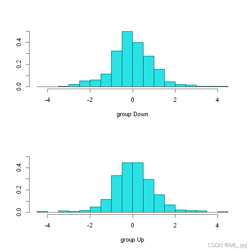
lda.pred <- predict(lda.fit, test)names(lda.pred)- 'class'
- 'posterior'
- 'x'
lda.class <- lda.pred$classtable(lda.class, test$Direction) lda.class Down Up Down 35 35 Up 76 106mean(lda.class == test$Direction)0.55952380952381
lda默认设置的阈值是0.5,即 P r ( d i r e c t i o n ∣ X = x ) > 0.5 = d o w n Pr(direction|X=x)>0.5 = down Pr(direction∣X=x)>0.5=down,可以通过lda.pred $ posterior调整重新计算lda.pred $ class
# 首先使用50%作为阈值sum(lda.pred$posterior[,1]>=0.5)70
sum(lda.pred$posterior[,1]<0.5)182
可以看出上述结果与lda默认得到的结果是一致的,假设我们更关注错把下降的预测为上升的,则可以调整更低的阈值,例如设置0.49为阈值
sum(lda.pred$posterior[,1]>=0.49)sum(lda.pred$posterior[,1]<0.49)147
105
此时结果有所不同
请注意,模型的后验概率输出对应于市场下降和上升的概率:
lda.pred$posterior[1:10,]| Down | Up | |
|---|---|---|
| 999 | 0.4901792 | 0.5098208 |
| 1000 | 0.4792185 | 0.5207815 |
| 1001 | 0.4668185 | 0.5331815 |
| 1002 | 0.4740011 | 0.5259989 |
| 1003 | 0.4927877 | 0.5072123 |
| 1004 | 0.4938562 | 0.5061438 |
| 1005 | 0.4951016 | 0.5048984 |
| 1006 | 0.4872861 | 0.5127139 |
| 1007 | 0.4907013 | 0.5092987 |
| 1008 | 0.4844026 | 0.5155974 |
4.4 二次判别分析
我们现在使用QDA模型拟合Smarket数据。QDA是在R中使用QDA()函数实现的,该函数也是MASS库的一部分。语法与lda()相同。
qda.fit <- qda(Direction ~ Lag1+Lag2, data=train)qda.fitCall:qda(Direction ~ Lag1 + Lag2, data = train)Prior probabilities of groups: DownUp 0.491984 0.508016 Group means: Lag1 Lag2Down 0.04279022 0.03389409Up -0.03954635 -0.03132544输出包含组平均值。但它不包含线性判别式的系数,因为QDA分类器涉及预测值的二次函数,而不是线性函数。predict()函数的工作方式与LDA完全相同。qda.class <- predict(qda.fit, test)$classtable(qda.class, test$Direction) qda.class Down Up Down 30 20 Up 81 121mean(qda.class == test$Direction)0.599206349206349
有趣的是,尽管2005年的数据没有用于拟合模型,但QDA的预测在几乎60%是准确的。对于股市数据来说,这种准确度已经很高,因为众所周知,股市数据很难准确建模。这表明,QDA假设的二次型可能比LDA和逻辑回归假设的线性型更准确地符合真实关系。然而,我们建在更大的测试集上评估这种方法的效果!
4.5 朴素贝叶斯
接下来,我们使用朴素贝叶斯拟合Smarket数据。在R中使用naiveBayes()函数实现,该函数是e1071库的一部分。语法与lda()和qda()相同。默认情况下,这种朴素贝叶斯分类器的实现使用高斯分布对每个定量特征进行建模。然而,核密度方法也可以用来估计分布。
library(e1071)nb.fit <- naiveBayes(Direction ~ Lag1 + Lag2, data = train)nb.fit
Naive Bayes Classifier for Discrete Predictors
Call:
naiveBayes.default(x = X, y = Y, laplace = laplace)
A-priori probabilities:Y DownUp 0.491984 0.508016 Conditional probabilities: Lag1Y [,1] [,2] Down 0.04279022 1.227446 Up -0.03954635 1.231668 Lag2Y [,1] [,2] Down 0.03389409 1.239191 Up -0.03132544 1.220765其中conditional probabilities表示条件分布的平均值和标准差
mean(train['Lag1'][train['Direction']=='Down'])0.0427902240325866
sd(train['Lag1'][train['Direction']=='Down'])1.22744562820108
predict()函数很简单
nb.class <- predict(nb.fit, test)table(nb.class, test$Direction) nb.class Down Up Down 28 20 Up 83 121mean(nb.class == test$Direction)0.591269841269841
Naive Bayes在这些数据上表现得非常好,准确预测率超过59%。这比QDA略差,但比LDA好得多
nb.preds <- predict(nb.fit, test,type = 'raw')nb.preds[1:5,]| Down | Up |
|---|---|
| 0.4873164 | 0.5126836 |
| 0.4762492 | 0.5237508 |
| 0.4653377 | 0.5346623 |
| 0.4748652 | 0.5251348 |
| 0.4901890 | 0.5098110 |
4.6 KNN
现在我们将使用KNN()函数执行KNN,该函数是class库的一部分。该函数的工作原理与我们迄今为止遇到的其他模型拟合函数截然不同。knn()不是一种参数估计方法,不是先拟合模型,然后使用模型进行预测,而是使用单个命令生成预测。该方法需要四个输入
- 包含与训练数据相关的预测变量的矩阵,标记为train.X.
- 一个矩阵,包含与我们希望对其进行预测的数据相关的预测值,标记为test.X.
- 包含训练观察的类标签的向量,标签为train.Direction.
- K的值,分类器使用的最近邻数。
我们使用cbind()函数(column bind的缩写)将lagone和lagtwo变量绑定到两个矩阵中,一个用于训练集,另一个用于测试集。
library(class)train.X <- cbind(train$Lag1,train$Lag2)test.X <- cbind(test$Lag1, test$Lag2)train.Direction <- train$DirectionWarning message:"package 'class' was built under R version 4.0.5"现在,knn()函数可以用来预测2005年的市场走势。在应用knn()之前,我们设置了一个随机种子,因为如果几个观测值作为最近邻并列,那么R将随机打破这种并列关系。因此,必须设定种子,以确保结果的可重复性。
set.seed(123)knn.pred <- knn(train.X, test.X, train.Direction, k = 1)table(knn.pred,test$Direction) knn.pred Down Up Down 43 58 Up 68 83mean(knn.pred == test$Direction)0.5
使用K=1的结果不是很好,因为只有50%的观测值被正确预测。当然,K=1可能会导致数据的拟合过于灵活。下面,我们使用K=3重复分析。
knn.pred <- knn(train.X, test.X, train.Direction, k = 3)table(knn.pred,test$Direction) knn.pred Down Up Down 48 55 Up 63 86mean(knn.pred == test$Direction)0.531746031746032
可以发现,正确率从50%上升到了53.17%.但事实证明,进一步增加K并不能带来进一步的改善。因为数据量不算大,对于这些数据,QDA提供了迄今为止我们研究过的方法中最好的结果。
KNN在Smarket数据上表现不佳,但它通常能提供令人印象深刻的结果。例如,我们将对保险数据集应用KNN方法,该数据集是ISLR2库的一部分。该数据集包括85个预测变量,用于测量5822个人的人口统计学特征。响应变量是Purchase,它表示给定的个人是否购买了商队保单。在这个数据集中,只有6%的人购买了商队保险。
dim(Caravan)- 5822
- 86
attach(Caravan)summary(Purchase)- No
- 5474
- 348
Yes
348 / 58220.0597732737890759
因为KNN分类器通过识别离它最近的观察值来预测给定测试观察值的类别,所以变量的量纲很重要。与小量纲变量相比,大量纲变量对观测值之间的距离以及KNN分类器的影响要大得多。处理这个问题的一个好方法是对数据进行标准化处理,使所有变量的平均值为零,标准偏差为1。然后所有变量都将处于可比较的范围内。scale()函数就是这样做的。在标准化数据时,我们排除了86列,因为这是定性购买变量。
#标准化处理standardized.X <- scale(Caravan[, -86])var(Caravan[, 1])165.037847395189
var(Caravan[, 2])0.164707781931954
var(standardized.X[, 1])1
var(standardized.X[, 2])可以看到标准化处理之后,不同变量的量纲一致
现在,我们将数据分为一个测试集(包含前1000个观察结果)和一个训练集(包含剩余的观察结果)。我们使用K=1在训练数据上拟合KNN模型,并在测试数据上评估其性能
test <- 1:1000train.X <- standardized.X[-test, ]test.X <- standardized.X[test, ]train.Y <- Purchase[-test]test.Y <- Purchase[test]set.seed(1)knn.pred <- knn(train.X, test.X, train.Y, k = 1)mean(test.Y != knn.pred)0.118
mean(test.Y != "No")0.059
table(knn.pred, test.Y) test.Yknn.pred No Yes No 873 50 Yes 68 9可以看出整体的拟合效果较好,但是预测为YES中只有9个数据预测正确,下面我们用K=3和K=5
knn.pred <- knn(train.X, test.X, train.Y, k = 3)table(knn.pred, test.Y) test.Yknn.pred No Yes No 920 54 Yes 21 55 / 260.192307692307692
knn.pred <- knn(train.X, test.X, train.Y, k = 5)table(knn.pred, test.Y) test.Yknn.pred No Yes No 930 55 Yes 11 44 / 150.266666666666667
glm.fits <- glm(Purchase ~ ., data = Caravan, family = binomial, subset = -test)Warning message:"glm.fit: fitted probabilities numerically 0 or 1 occurred"glm.probs <- predict(glm.fits, Caravan[test, ], type = "response")glm.pred .5] <- "Yes"table(glm.pred, test.Y) test.Yglm.pred No Yes No 934 59 Yes 7 0glm.pred .25] <- "Yes"table(glm.pred, test.Y) test.Yglm.pred No Yes No 919 48 Yes 22 114.7 泊松回归
最后,我们将泊松回归模型拟合Bikeshare数据集,该数据集测量华盛顿特区每小时的自行车租赁(骑自行车者)数量。这些数据可以在ISLR2库中找到。
attach(Bikeshare)dim(Bikeshare)- 8645
- 15
names(Bikeshare)- 'season'
- 'mnth'
- 'day'
- 'hr'
- 'holiday'
- 'weekday'
- 'workingday'
- 'weathersit'
- 'temp'
- 'atemp'
- 'hum'
- 'windspeed'
- 'casual'
- 'registered'
- 'bikers'
我们首先用最小二乘线性回归模型拟合数据。
mod.lm <- lm( bikers ~ mnth + hr + workingday + temp + weathersit, data = Bikeshare)summary(mod.lm)
Call:
lm(formula = bikers ~ mnth + hr + workingday + temp + weathersit,
data = Bikeshare)
Residuals:
Min 1Q Median 3Q Max
-299.00 -45.70 -6.23 41.08 425.29
Coefficients: Estimate Std. Error t value Pr(>|t|) (Intercept) 73.5974 5.1322 14.340 < 2e-16 ***mnth1 -46.0871 4.0855 -11.281 < 2e-16 ***mnth2 -39.2419 3.5391 -11.088 < 2e-16 ***mnth3 -29.5357 3.1552 -9.361 < 2e-16 ***mnth4 -4.6622 2.7406 -1.701 0.08895 . mnth5 26.4700 2.8508 9.285 < 2e-16 ***mnth6 21.7317 3.4651 6.272 3.75e-10 ***mnth7 -0.7626 3.9084 -0.195 0.84530 mnth8 7.1560 3.5347 2.024 0.04295 * mnth9 20.5912 3.0456 6.761 1.46e-11 ***mnth10 29.7472 2.6995 11.019 < 2e-16 ***mnth11 14.2229 2.8604 4.972 6.74e-07 ***hr1 -96.1420 3.9554 -24.307 < 2e-16 ***hr2 -110.7213 3.9662 -27.916 < 2e-16 ***hr3 -117.7212 4.0165 -29.310 < 2e-16 ***hr4 -127.2828 4.0808 -31.191 < 2e-16 ***hr5 -133.0495 4.1168 -32.319 < 2e-16 ***hr6 -120.2775 4.0370 -29.794 < 2e-16 ***hr7 -75.5424 3.9916 -18.925 < 2e-16 ***hr8 23.9511 3.9686 6.035 1.65e-09 ***hr9 127.5199 3.9500 32.284 < 2e-16 ***hr10 24.4399 3.9360 6.209 5.57e-10 ***hr11 -12.3407 3.9361 -3.135 0.00172 ** hr12 9.2814 3.9447 2.353 0.01865 * hr13 41.1417 3.9571 10.397 < 2e-16 ***hr14 39.8939 3.9750 10.036 < 2e-16 ***hr15 30.4940 3.9910 7.641 2.39e-14 ***hr16 35.9445 3.9949 8.998 < 2e-16 ***hr17 82.3786 3.9883 20.655 < 2e-16 ***hr18 200.1249 3.9638 50.488 < 2e-16 ***hr19 173.2989 3.9561 43.806 < 2e-16 ***hr20 90.1138 3.9400 22.872 < 2e-16 ***hr21 29.4071 3.9362 7.471 8.74e-14 ***hr22 -8.5883 3.9332 -2.184 0.02902 * hr23 -37.0194 3.9344 -9.409 < 2e-16 ***workingday 1.2696 1.7845 0.711 0.47681 temp 157.2094 10.2612 15.321 < 2e-16 ***weathersitcloudy/misty -12.8903 1.9643 -6.562 5.60e-11 ***weathersitlight rain/snow -66.4944 2.9652 -22.425 < 2e-16 ***weathersitheavy rain/snow -109.7446 76.6674 -1.431 0.15234 ---Signif. codes: 0 '***' 0.001 '**' 0.01 '*' 0.05 '.' 0.1 ' ' 1Residual standard error: 76.5 on 8605 degrees of freedomMultiple R-squared: 0.6745,Adjusted R-squared: 0.6731 F-statistic: 457.3 on 39 and 8605 DF, p-value: < 2.2e-16在hr(0)和mnth(Jan)的视为基础值,因此没有为它们提供系数估计。也就是题目的系数估计为0,其他的系数都是基于这个基础
下面我们做一些细微的调整,对hr和mnth取虚拟变量,结果如下
contrasts(Bikeshare$hr) = contr.sum(24)contrasts(Bikeshare$mnth) = contr.sum(12)mod.lm2 <- lm( bikers ~ mnth + hr + workingday + temp + weathersit, data = Bikeshare )summary(mod.lm2)
Call:
lm(formula = bikers ~ mnth + hr + workingday + temp + weathersit,
data = Bikeshare)
Residuals:
Min 1Q Median 3Q Max
-299.00 -45.70 -6.23 41.08 425.29
Coefficients: Estimate Std. Error t value Pr(>|t|) (Intercept) 73.5974 5.1322 14.340 < 2e-16 ***mnth1 -46.0871 4.0855 -11.281 < 2e-16 ***mnth2 -39.2419 3.5391 -11.088 < 2e-16 ***mnth3 -29.5357 3.1552 -9.361 < 2e-16 ***mnth4 -4.6622 2.7406 -1.701 0.08895 . mnth5 26.4700 2.8508 9.285 < 2e-16 ***mnth6 21.7317 3.4651 6.272 3.75e-10 ***mnth7 -0.7626 3.9084 -0.195 0.84530 mnth8 7.1560 3.5347 2.024 0.04295 * mnth9 20.5912 3.0456 6.761 1.46e-11 ***mnth10 29.7472 2.6995 11.019 < 2e-16 ***mnth11 14.2229 2.8604 4.972 6.74e-07 ***hr1 -96.1420 3.9554 -24.307 < 2e-16 ***hr2 -110.7213 3.9662 -27.916 < 2e-16 ***hr3 -117.7212 4.0165 -29.310 < 2e-16 ***hr4 -127.2828 4.0808 -31.191 < 2e-16 ***hr5 -133.0495 4.1168 -32.319 < 2e-16 ***hr6 -120.2775 4.0370 -29.794 < 2e-16 ***hr7 -75.5424 3.9916 -18.925 < 2e-16 ***hr8 23.9511 3.9686 6.035 1.65e-09 ***hr9 127.5199 3.9500 32.284 < 2e-16 ***hr10 24.4399 3.9360 6.209 5.57e-10 ***hr11 -12.3407 3.9361 -3.135 0.00172 ** hr12 9.2814 3.9447 2.353 0.01865 * hr13 41.1417 3.9571 10.397 < 2e-16 ***hr14 39.8939 3.9750 10.036 < 2e-16 ***hr15 30.4940 3.9910 7.641 2.39e-14 ***hr16 35.9445 3.9949 8.998 < 2e-16 ***hr17 82.3786 3.9883 20.655 < 2e-16 ***hr18 200.1249 3.9638 50.488 < 2e-16 ***hr19 173.2989 3.9561 43.806 < 2e-16 ***hr20 90.1138 3.9400 22.872 < 2e-16 ***hr21 29.4071 3.9362 7.471 8.74e-14 ***hr22 -8.5883 3.9332 -2.184 0.02902 * hr23 -37.0194 3.9344 -9.409 < 2e-16 ***workingday 1.2696 1.7845 0.711 0.47681 temp 157.2094 10.2612 15.321 < 2e-16 ***weathersitcloudy/misty -12.8903 1.9643 -6.562 5.60e-11 ***weathersitlight rain/snow -66.4944 2.9652 -22.425 < 2e-16 ***weathersitheavy rain/snow -109.7446 76.6674 -1.431 0.15234 ---Signif. codes: 0 '***' 0.001 '**' 0.01 '*' 0.05 '.' 0.1 ' ' 1Residual standard error: 76.5 on 8605 degrees of freedomMultiple R-squared: 0.6745,Adjusted R-squared: 0.6731 F-statistic: 457.3 on 39 and 8605 DF, p-value: < 2.2e-16两个模型之间的区别
在模型2中,mnth和hr的最后一个水平不等于0,它是其他系数的总和的相反数,也就是说,hr和mnth所有取值系数的和会等于0,因此单个系数可以解释为与平均水平相比
重要的是要认识到,如果我们根据使用的编码正确解释模型输出,编码的选择实际上并不重要。例如,我们看到,无论编码如何,线性模型的预测都是相同的:
sum((predict(mod.lm) - predict(mod.lm2))^2)0
all.equal(predict(mod.lm), predict(mod.lm2))TRUE
为了画出图4.13左边的图,我们必须首先获得与mnth相关的系数估计。
1月至11月的系数可直接从模型结果获得。12月份的系数必须明确计算为所有其他月份的和的相反数。
coef.months <- c(coef(mod.lm2)[2:12], -sum(coef(mod.lm2)[2:12]))plot(coef.months, xlab = "Month", ylab = "Coefficient", xaxt = "n", col = "blue", pch = 19, type = "o")axis(side = 1, at = 1:12, labels = c("J", "F", "M", "A", "M", "J", "J", "A", "S", "O", "N", "D"))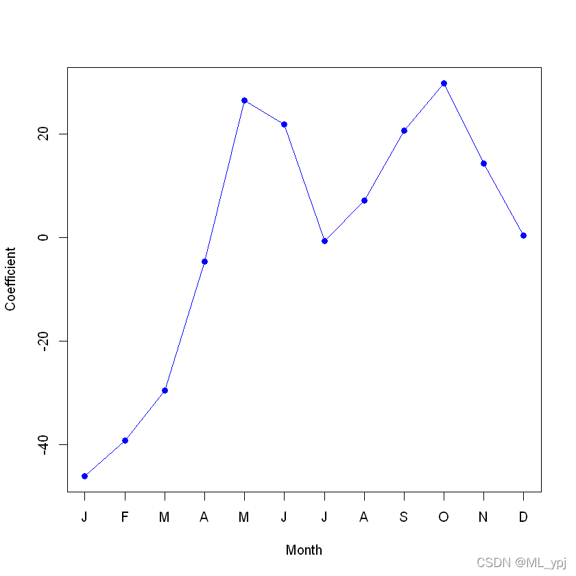
同理画出图4.13右图
coef.hours <- c(coef(mod.lm2)[13:35], -sum(coef(mod.lm2)[13:35]))plot(coef.hours, xlab = "Hour", ylab = "Coefficient", col = "blue", pch = 19, type = "o")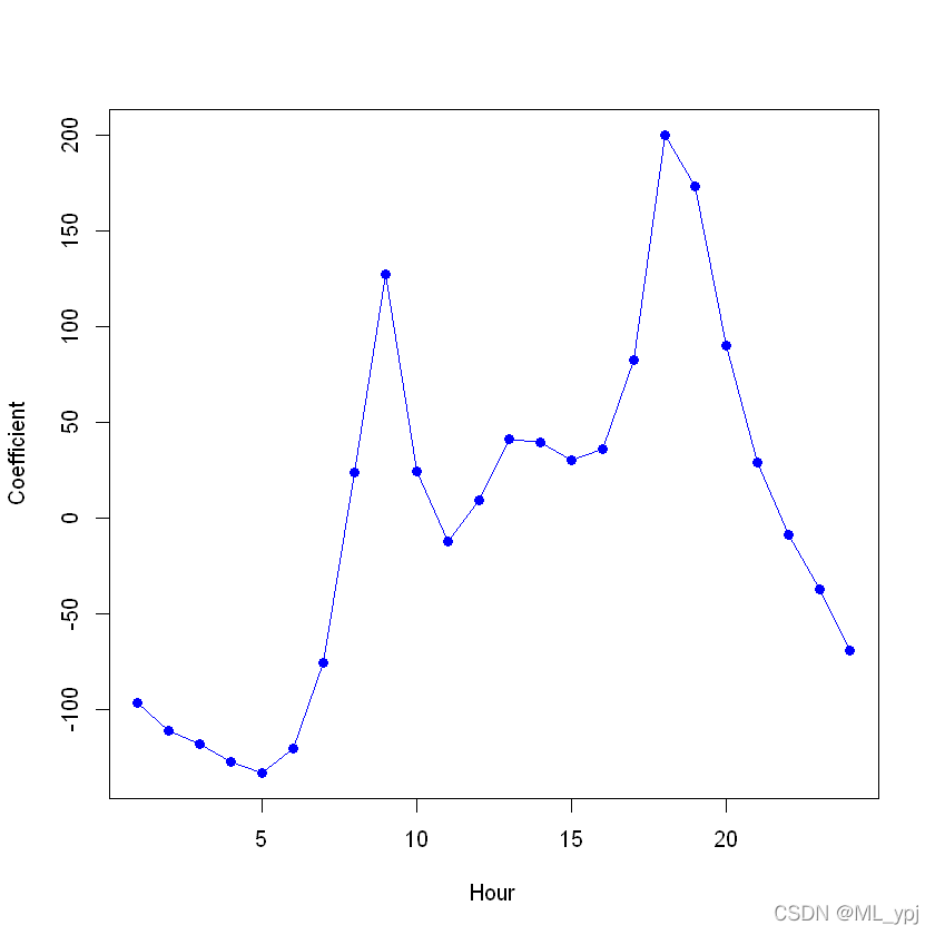
现在,我们考虑将泊松回归模型拟合到Bikeshayes数据。
除了我们现在使用参数family=poisson的函数glm()来指定我们希望拟合泊松回归模型之外,几乎没有什么变化:
mod.pois <- glm( bikers ~ mnth+hr+workingday+temp+ weathersit, data = Bikeshare, family = poisson)summary(mod.pois)
Call:
glm(formula = bikers ~ mnth + hr + workingday + temp + weathersit,
family = poisson, data = Bikeshare)
Deviance Residuals:
Min 1Q Median 3Q Max
-20.7574 -3.3441 -0.6549 2.6999 21.9628
Coefficients: Estimate Std. Error z value Pr(>|z|) (Intercept) 4.118245 0.006021 683.964 < 2e-16 ***mnth1-0.670170 0.005907 -113.445 < 2e-16 ***mnth2-0.444124 0.004860 -91.379 < 2e-16 ***mnth3-0.293733 0.004144 -70.886 < 2e-16 ***mnth4 0.021523 0.003125 6.888 5.66e-12 ***mnth5 0.240471 0.002916 82.462 < 2e-16 ***mnth6 0.223235 0.003554 62.818 < 2e-16 ***mnth7 0.103617 0.004125 25.121 < 2e-16 ***mnth8 0.151171 0.003662 41.281 < 2e-16 ***mnth9 0.233493 0.003102 75.281 < 2e-16 ***mnth100.267573 0.002785 96.091 < 2e-16 ***mnth110.150264 0.003180 47.248 < 2e-16 ***hr1 -0.754386 0.007879 -95.744 < 2e-16 ***hr2 -1.225979 0.009953 -123.173 < 2e-16 ***hr3 -1.563147 0.011869 -131.702 < 2e-16 ***hr4 -2.198304 0.016424 -133.846 < 2e-16 ***hr5 -2.830484 0.022538 -125.586 < 2e-16 ***hr6 -1.814657 0.013464 -134.775 < 2e-16 ***hr7 -0.429888 0.006896 -62.341 < 2e-16 ***hr8 0.575181 0.004406 130.544 < 2e-16 ***hr9 1.076927 0.003563 302.220 < 2e-16 ***hr10 0.581769 0.004286 135.727 < 2e-16 ***hr11 0.336852 0.004720 71.372 < 2e-16 ***hr12 0.494121 0.004392 112.494 < 2e-16 ***hr13 0.679642 0.004069 167.040 < 2e-16 ***hr14 0.673565 0.004089 164.722 < 2e-16 ***hr15 0.624910 0.004178 149.570 < 2e-16 ***hr16 0.653763 0.004132 158.205 < 2e-16 ***hr17 0.874301 0.003784 231.040 < 2e-16 ***hr18 1.294635 0.003254 397.848 < 2e-16 ***hr19 1.212281 0.003321 365.084 < 2e-16 ***hr20 0.914022 0.003700 247.065 < 2e-16 ***hr21 0.616201 0.004191 147.045 < 2e-16 ***hr22 0.364181 0.004659 78.173 < 2e-16 ***hr23 0.117493 0.005225 22.488 < 2e-16 ***workingday 0.014665 0.001955 7.502 6.27e-14 ***temp 0.785292 0.011475 68.434 < 2e-16 ***weathersitcloudy/misty -0.075231 0.002179 -34.528 < 2e-16 ***weathersitlight rain/snow -0.575800 0.004058 -141.905 < 2e-16 ***weathersitheavy rain/snow -0.926287 0.166782 -5.554 2.79e-08 ***---Signif. codes: 0 '***' 0.001 '**' 0.01 '*' 0.05 '.' 0.1 ' ' 1(Dispersion parameter for poisson family taken to be 1) Null deviance: 1052921 on 8644 degrees of freedomResidual deviance: 228041 on 8605 degrees of freedomAIC: 281159Number of Fisher Scoring iterations: 5我们可以绘制与mnth和hr相关的系数,以重现图4.15:
coef.mnth <- c(coef(mod.pois)[2:12], -sum(coef(mod.pois)[2:12]))plot(coef.mnth, xlab = "Month", ylab = "Coefficient", xaxt = "n", col = "blue", pch = 19, type = "o")axis(side = 1, at = 1:12, labels = c("J", "F", "M", "A", "M", "J", "J", "A", "S", "O", "N", "D"))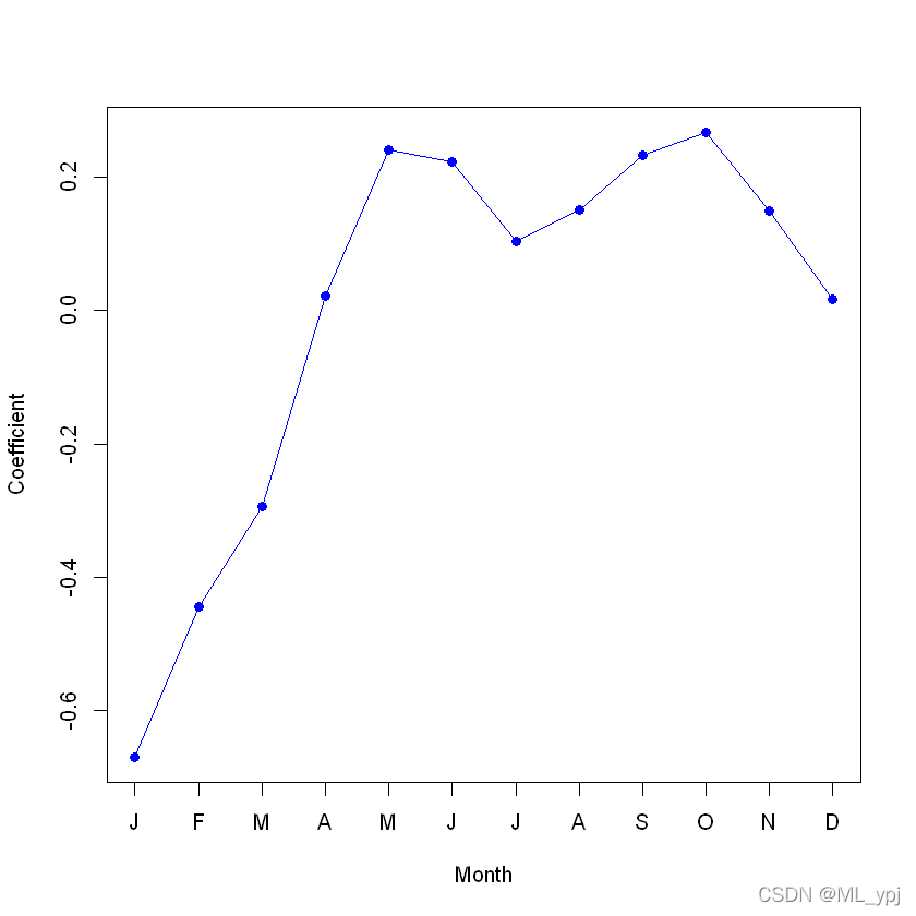
coef.hours <- c(coef(mod.pois)[13:35], -sum(coef(mod.pois)[13:35]))plot(coef.hours, xlab = "Hour", ylab = "Coefficient", col = "blue", pch = 19, type = "o")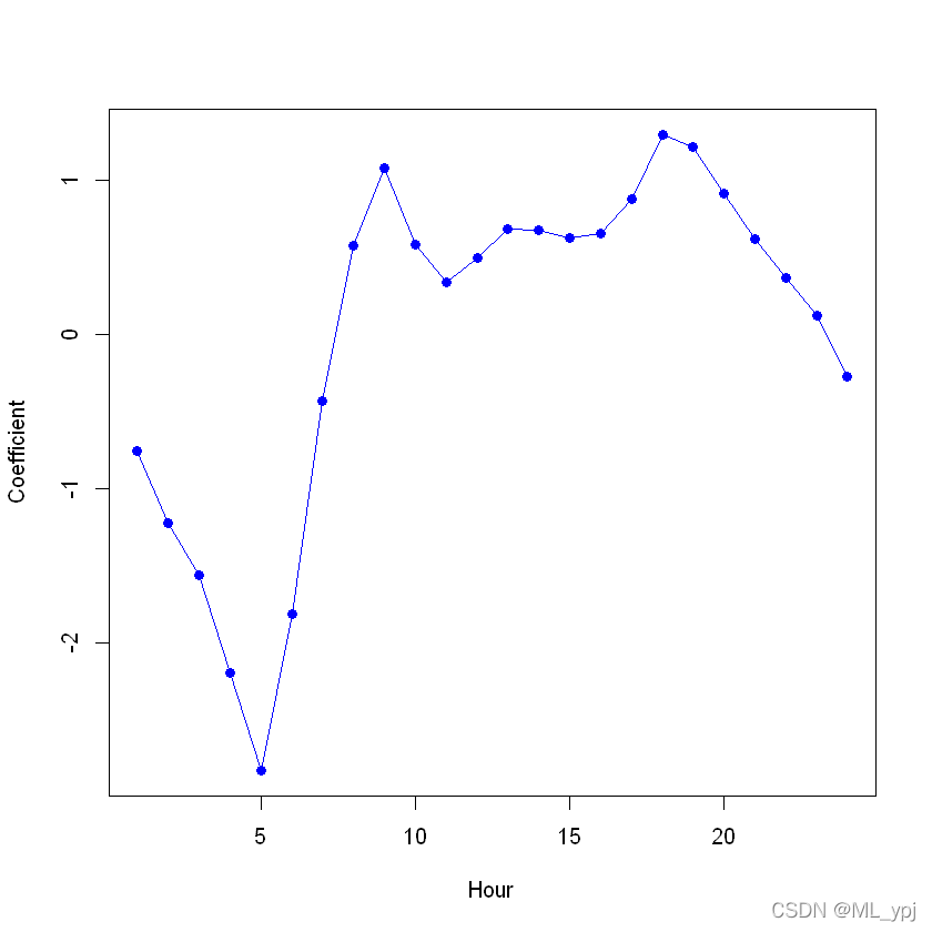
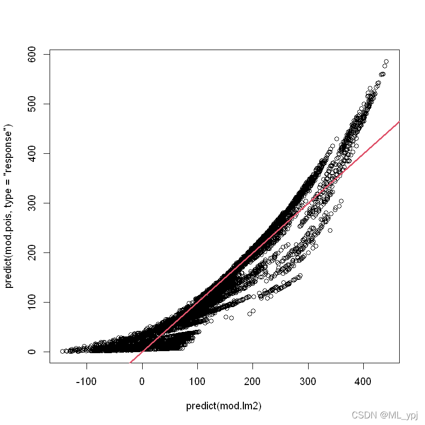
现在我们可以再次使用predict()函数从泊松回归模型中得到拟合值。在这里,我们必须指定参数type='response'给R,
让输出是 e x p ( β ^ 0 + β ^ 1 X1 + . . . + β ^ p Xp ) exp({\hat{\beta}_0+\hat{\beta}_1X_1+...+\hat{\beta}_pX_p}) exp(β^0+β^1X1+...+β^pXp)而不是β^ 0 + β^ 1 X 1 + . . . + β^ p X p \hat{\beta}_0+\hat{\beta}_1X_1+...+\hat{\beta}_pX_p β^0+β^1X1+...+β^pXp
plot(predict(mod.lm2), predict(mod.pois, type = "response"))abline(0, 1, col = 2, lwd = 3)