统计学习导论(ISLR)

---

参考资料:
The Elements of Statistical Learning
An Introduction to Statistical Learning
统计学习导论（ISLR）（二）：统计学习概述
统计学习导论（ISLR）（三）：线性回归
统计学习导论（ISLR）（四）：分类
统计学习导论（ISLR）（五）：重采样方法（交叉验证和boostrap）
ISLR统计学习导论之R语言应用（二）：R语言基础
ISLR统计学习导论之R语言应用（三）：线性回归R语言代码实战
ISLR统计学习导论之R语言应用（四）：分类算法R语言代码实战
ISLR统计学习导论之R语言应用（五）：R语言实现交叉验证和bootstrap
统计学习导论（ISLR） 第三章课后习题
统计学习导论（ISLR） 第四章课后习题
统计学习导论（ISLR）第五章课后习题

文章目录

• 统计学习导论(ISLR)
• 第三章 线性回归课后题
• 8. 这个问题涉及在Auto数据集上使用简单线性回归。
• • a 使用lm（）函数执行简单的线性回归，以mpg作为响应，horsepower作为预测变量。使用summary（）函数输出结果。对输出进行分析。例如：
  • Answer:
  • b 绘制响应和预测值散点图。使用abline()函数显示最小二乘回归线。
  • c
• 9 使用Auto数据集进行多元线性回归
• • (a)生成包含数据集中所有变量的散点图矩阵
  • b使用函数cor（）计算变量之间的相关性矩阵。首先排除name变量，因为他是定性变量
  • c.使用lm()函数拟合多元线性回归模型，使用除了name以外的所有变量
  • d. 通过plot()函数得到该模型的结果分析
  • e使用*和：产生回归交互项，观察使用这些交互项是否对模型拟合效果有帮助
  • f.尝试对预测变量进行一些不同的变化来拟合模型
• 10.使用Carseats数据集拟合模型
• • a.使用price，urban，us拟合多元线性回归预测sales
  • b.分析各个变量对Sales的影响
  • c 写出模型的等式关系
  • d
  • e
  • f.
  • g.
  • h.拟合结果是否存在离群值和高杠杆点
• 11.
• • a 根据模拟数据拟合y对x简单的线性回归模型，没有截距项
  • b.拟合x对y的线性回归，依然没有截距
  • c
  • d
  • e
  • f
• 12
• • a.
  • b.回归系数不等的例子
  • c.回归系数相等的例子
• 13
• • a.
  • b
  • c
  • e
  • f
  • g
  • h
  • i
  • j
• 14
• • a
  • b
  • c
  • d
  • e
  • f
  • g

---

第三章 线性回归课后题

8. 这个问题涉及在Auto数据集上使用简单线性回归。

a 使用lm（）函数执行简单的线性回归，以mpg作为响应，horsepower作为预测变量。使用summary（）函数输出结果。对输出进行分析。例如：

• 预测因子和响应之间有关系吗？
• 预测因子和响应之间的关系有多强？
• 预测因子和响应之间的关系是正的还是负的？
• 给定horsepower=98，mpg的置信区间和预测区间

# 导入基本库library(ISLR2)lm1 = lm(mpg~horsepower, data=Auto)

summary(lm1)

​

Call:lm(formula = mpg ~ horsepower, data = Auto)Residuals:     Min1Q   Median3Q      Max -13.5710  -3.2592  -0.3435   2.7630  16.9240 Coefficients:      Estimate Std. Error t value Pr(>|t|)    (Intercept) 39.935861   0.717499   55.66   <2e-16 ***horsepower  -0.157845   0.006446  -24.49   <2e-16 ***---Signif. codes:  0 '***' 0.001 '**' 0.01 '*' 0.05 '.' 0.1 ' ' 1Residual standard error: 4.906 on 390 degrees of freedomMultiple R-squared:  0.6059,Adjusted R-squared:  0.6049 F-statistic: 599.7 on 1 and 390 DF,  p-value: < 2.2e-16

Answer:

1)从输出结果可以看出，t检验对于的p值<0.05,mpg与horsepower之间存在显著的线性关系
2) R 2 = 0.6059 R^2 = 0.6059 R2=0.6059,这表明mpg中60.5948%的方差由horsepower解释
3)horsepower的系数为-0.1579，说明两者之间是负相关，即horsepower越高，mpg越低

4)计算不同置信水平下的置信区间

# 计算置信区间predict(lm1, data.frame(horsepower=c(98)), interval = 'confidence')

A matrix: 1 × 3 of type dbl

	fit	lwr	upr
1	24.46708	23.97308	24.96108

# 计算预测区间predict(lm1, data.frame(horsepower=c(99)), interval = 'prediction')

A matrix: 1 × 3 of type dbl

	fit	lwr	upr
1	24.30923	14.65165	33.96681

可以看出预测区间大于置信区间，这可以从两个区间的计算公式得出

b 绘制响应和预测值散点图。使用abline()函数显示最小二乘回归线。

plot(horsepower, mpg)abline(lm1, col = 'red',lwd = 2)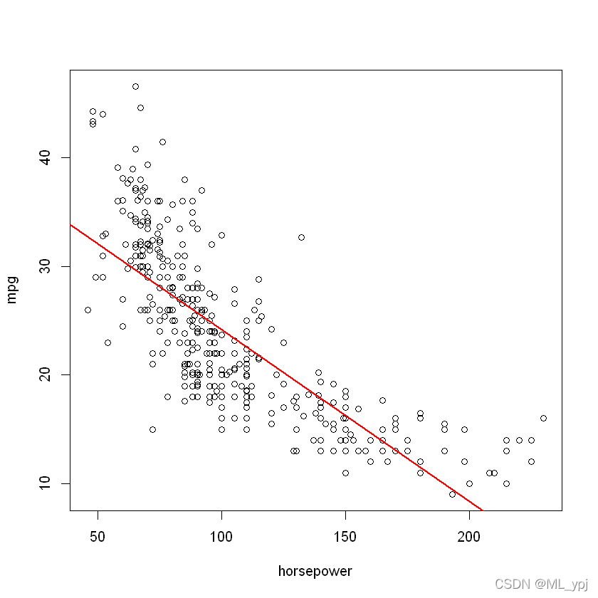

c

使用Plot（）函数生成最小二乘回归拟合的诊断图。并分析

par(mfrow=c(2,2))plot(lm1)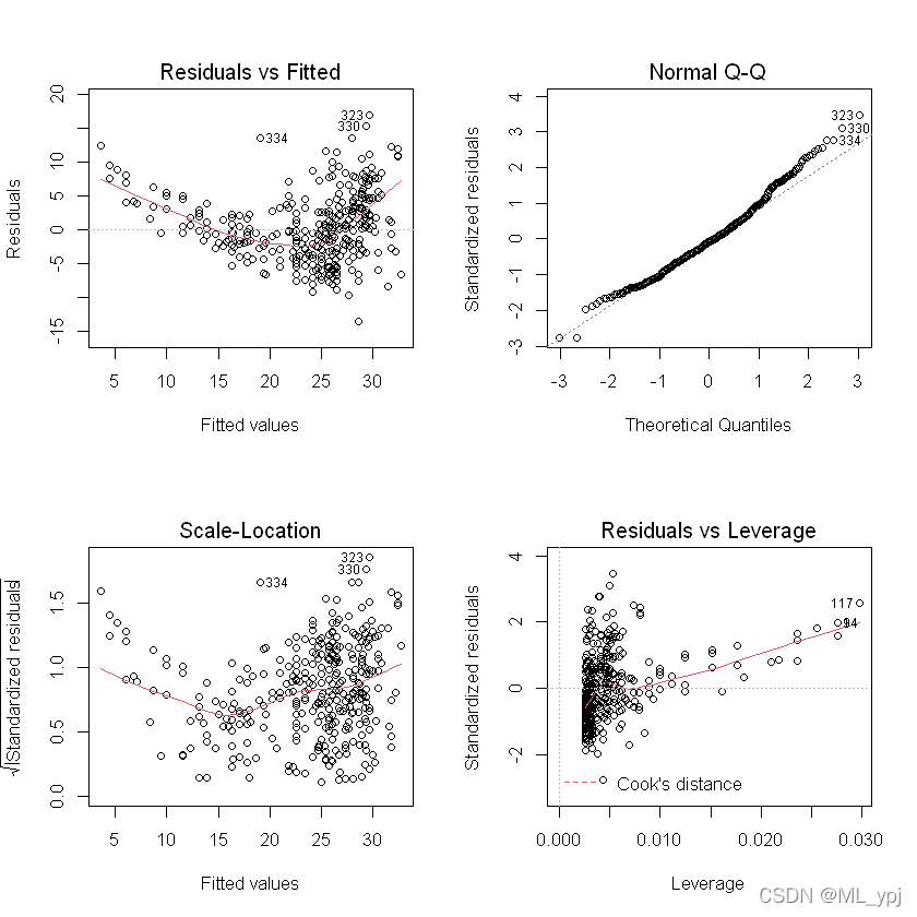

从残差图可以看出，存在一定的非线性趋势。

9 使用Auto数据集进行多元线性回归

(a)生成包含数据集中所有变量的散点图矩阵

pairs(Auto)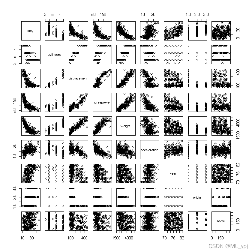

b使用函数cor（）计算变量之间的相关性矩阵。首先排除name变量，因为他是定性变量

# 计算变量相关系数矩阵，去除name变量cor(subset(Auto, select = -name))

A matrix: 8 × 8 of type dbl

	mpg	cylinders	displacement	horsepower	weight	acceleration	year	origin
mpg	1.0000000	-0.7776175	-0.8051269	-0.7784268	-0.8322442	0.4233285	0.5805410	0.5652088
cylinders	-0.7776175	1.0000000	0.9508233	0.8429834	0.8975273	-0.5046834	-0.3456474	-0.5689316
displacement	-0.8051269	0.9508233	1.0000000	0.8972570	0.9329944	-0.5438005	-0.3698552	-0.6145351
horsepower	-0.7784268	0.8429834	0.8972570	1.0000000	0.8645377	-0.6891955	-0.4163615	-0.4551715
weight	-0.8322442	0.8975273	0.9329944	0.8645377	1.0000000	-0.4168392	-0.3091199	-0.5850054
acceleration	0.4233285	-0.5046834	-0.5438005	-0.6891955	-0.4168392	1.0000000	0.2903161	0.2127458
year	0.5805410	-0.3456474	-0.3698552	-0.4163615	-0.3091199	0.2903161	1.0000000	0.1815277
origin	0.5652088	-0.5689316	-0.6145351	-0.4551715	-0.5850054	0.2127458	0.1815277	1.0000000

c.使用lm()函数拟合多元线性回归模型，使用除了name以外的所有变量

lm2 = lm(mpg~.-name, data=Auto)summary(lm2)

​

Call:lm(formula = mpg ~ . - name, data = Auto)Residuals:    Min      1Q  Median      3Q     Max -9.5903 -2.1565 -0.1169  1.8690 13.0604 Coefficients: Estimate Std. Error t value Pr(>|t|)    (Intercept)  -17.218435   4.644294  -3.707  0.00024 ***cylinders     -0.493376   0.323282  -1.526  0.12780    displacement   0.019896   0.007515   2.647  0.00844 ** horsepower    -0.016951   0.013787  -1.230  0.21963    weight -0.006474   0.000652  -9.929  < 2e-16 ***acceleration   0.080576   0.098845   0.815  0.41548    year    0.750773   0.050973  14.729  < 2e-16 ***origin  1.426141   0.278136   5.127 4.67e-07 ***---Signif. codes:  0 '***' 0.001 '**' 0.01 '*' 0.05 '.' 0.1 ' ' 1Residual standard error: 3.328 on 384 degrees of freedomMultiple R-squared:  0.8215,Adjusted R-squared:  0.8182 F-statistic: 252.4 on 7 and 384 DF,  p-value: < 2.2e-16

• 1模型整体是显著的
• 2 变量 displacement、weight、year、origin是显著的
• 3从year的回归系数得出，每增加一年，mpg增加0.75个单位

d. 通过plot()函数得到该模型的结果分析

par(mfrow=c(2,2))plot(lm2)

由于残差图中存在曲线模式，因此线性回归拟合准确。从杠杆率图来看，点14似乎具有较高的杠杆率，尽管剩余量不高。

plot(predict(lm2), rstudent(lm2))

学生化残差图中存在异常值，因为存在值大于3的数据。

e使用*和：产生回归交互项，观察使用这些交互项是否对模型拟合效果有帮助

这里我们使用各个显著的四个变量：displacement、weight、year、origin，以及displacement和year的交互项进行分析

：表示两个变量的交互项
$\ast$：不仅包括交互项，还包括他们原来的线性模型， x 1 ∗ x 2 = x 1 + x 2 + x 1 : x 2 x_1*x_2=x_1+x_2+x_1:x_2 x1​∗x2​=x1​+x2​+x1​:x2​

lm3 <- lm(mpg~displacement*year+weight+origin,data=Auto)summary(lm3)

​

Call:lm(formula = mpg ~ displacement * year + weight + origin, data = Auto)Residuals:    Min      1Q  Median      3Q     Max -8.9697 -1.9596  0.0146  1.5575 13.0308 Coefficients:      Estimate Std. Error t value Pr(>|t|)    (Intercept)-5.733e+01  7.289e+00  -7.864 3.75e-14 ***displacement2.228e-01  3.504e-02   6.358 5.78e-10 ***year 1.287e+00  9.514e-02  13.524  < 2e-16 ***weight     -6.080e-03  5.374e-04 -11.313  < 2e-16 ***origin      9.755e-01  2.579e-01   3.783  0.00018 ***displacement:year -2.989e-03  4.782e-04  -6.251 1.08e-09 ***---Signif. codes:  0 '***' 0.001 '**' 0.01 '*' 0.05 '.' 0.1 ' ' 1Residual standard error: 3.193 on 386 degrees of freedomMultiple R-squared:  0.8348,Adjusted R-squared:  0.8327 F-statistic: 390.2 on 5 and 386 DF,  p-value: < 2.2e-16

par(mfrow=c(2,2))plot(lm3)

从残差图来看，拟合的结果比没有交互项的模型有了一定的提升

f.尝试对预测变量进行一些不同的变化来拟合模型

lm4 <- lm(mpg~displacement+year+weight+sqrt(origin),data=Auto)

par(mfrow = c(2,2))plot(lm4)

lm5 <- lm(mpg~displacement+year+weight+I(origin^2),data=Auto)

par(mfrow = c(2,2))plot(lm5)

10.使用Carseats数据集拟合模型

a.使用price，urban，us拟合多元线性回归预测sales

# 加载数据集attach(Carseats)

# 拟合模型lm.fit <- lm(Sales~Price+Urban+US, data = Carseats)summary(lm.fit)

​

Call:lm(formula = Sales ~ Price + Urban + US, data = Carseats)Residuals:    Min      1Q  Median      3Q     Max -6.9206 -1.6220 -0.0564  1.5786  7.0581 Coefficients:      Estimate Std. Error t value Pr(>|t|)    (Intercept) 13.043469   0.651012  20.036  < 2e-16 ***Price-0.054459   0.005242 -10.389  < 2e-16 ***UrbanYes    -0.021916   0.271650  -0.081    0.936    USYes 1.200573   0.259042   4.635 4.86e-06 ***---Signif. codes:  0 '***' 0.001 '**' 0.01 '*' 0.05 '.' 0.1 ' ' 1Residual standard error: 2.472 on 396 degrees of freedomMultiple R-squared:  0.2393,Adjusted R-squared:  0.2335 F-statistic: 41.52 on 3 and 396 DF,  p-value: < 2.2e-16

b.分析各个变量对Sales的影响

• price:价格变量通过了显著性检验，并且相关系数为负，说明价格越高销售量越低
• UrbanYes：变量没有通过显著性检验，说明是否在城市对于销售量没有显著的影响
• USYes：变量通过了显著性检验，并且相关系数为1.20，这说明如果在美国销售量会增加1201个单位

c 写出模型的等式关系

$Sales=13.04-0.05Price-0.02UrbanYes+1.20USYes$

d

通过p值可以判断Price和USYes通过了显著性检验

e

只使用price和US两个变量拟合模型

lm.fit2 <- lm(Sales~US+Price, data = Carseats)summary(lm.fit2)

​

Call:lm(formula = Sales ~ US + Price, data = Carseats)Residuals:    Min      1Q  Median      3Q     Max -6.9269 -1.6286 -0.0574  1.5766  7.0515 Coefficients:     Estimate Std. Error t value Pr(>|t|)    (Intercept) 13.03079    0.63098  20.652  < 2e-16 ***USYes 1.19964    0.25846   4.641 4.71e-06 ***Price-0.05448    0.00523 -10.416  < 2e-16 ***---Signif. codes:  0 '***' 0.001 '**' 0.01 '*' 0.05 '.' 0.1 ' ' 1Residual standard error: 2.469 on 397 degrees of freedomMultiple R-squared:  0.2393,Adjusted R-squared:  0.2354 F-statistic: 62.43 on 2 and 397 DF,  p-value: < 2.2e-16

f.

从RSE和R方来看e中的模型更好

g.

求相关系数的95%的置信区间

confint(lm.fit2)

A matrix: 3 × 2 of type dbl

	2.5 %	97.5 %
(Intercept)	11.79032020	14.27126531
USYes	0.69151957	1.70776632
Price	-0.06475984	-0.04419543

h.拟合结果是否存在离群值和高杠杆点

plot(predict(lm.fit2), rstudent(lm.fit2))

从上图结果来看，所有值都在-3和3之间，没有离群点

Error in parse(text = x, srcfile = src): :1:15: unexpected input1: 从上图结果来看，    ^Traceback:

par(mfrow = c(2,2))plot(lm.fit2)

从上图来看，存在高杠杆值

11.

set.seed(1)x <- rnorm(100)y <- 2*x + rnorm(100)

a 根据模拟数据拟合y对x简单的线性回归模型，没有截距项

lm.fit <- lm(y~x+0, data=data.frame(x,y))summary(lm.fit)

​

Call:lm(formula = y ~ x + 0, data = data.frame(x, y))Residuals:    Min      1Q  Median      3Q     Max -1.9154 -0.6472 -0.1771  0.5056  2.3109 Coefficients:  Estimate Std. Error t value Pr(>|t|)    x   1.9939     0.1065   18.73   <2e-16 ***---Signif. codes:  0 '***' 0.001 '**' 0.01 '*' 0.05 '.' 0.1 ' ' 1Residual standard error: 0.9586 on 99 degrees of freedomMultiple R-squared:  0.7798,Adjusted R-squared:  0.7776 F-statistic: 350.7 on 1 and 99 DF,  p-value: < 2.2e-16

t检验的p值解决0，因此我们拒绝原假设

b.拟合x对y的线性回归，依然没有截距

lm.fit <- lm(x~y+0)summary(lm.fit)

​

Call:lm(formula = x ~ y + 0)Residuals:    Min      1Q  Median      3Q     Max -0.8699 -0.2368  0.1030  0.2858  0.8938 Coefficients:  Estimate Std. Error t value Pr(>|t|)    y  0.39111    0.02089   18.73   <2e-16 ***---Signif. codes:  0 '***' 0.001 '**' 0.01 '*' 0.05 '.' 0.1 ' ' 1Residual standard error: 0.4246 on 99 degrees of freedomMultiple R-squared:  0.7798,Adjusted R-squared:  0.7776 F-statistic: 350.7 on 1 and 99 DF,  p-value: < 2.2e-16

同样p值接近0，拒绝原假设

c

从a和b的结果可以得出 $y=2x+ϵ$可以写成$x=0.5(y-ϵ)$

d

(sqrt(length(x)-1) * sum(x*y)) / (sqrt(sum(x*x) * sum(y*y) - (sum(x*y))^2))

18.7259319374486

e

结果是一样的

f

从上述两个回归结果来看，t统计量的值是一样的

12

a.

当x观测值的平方和等于y观测值的平方和时，回归系数相等

b.回归系数不等的例子

set.seed(1)x = rnorm(100)y = 2*xlm.fit = lm(y~x+0)lm.fit2 = lm(x~y+0)summary(lm.fit)

Warning message in summary.lm(lm.fit):"essentially perfect fit: summary may be unreliable"Call:lm(formula = y ~ x + 0)Residuals:Min  1Q     Median  3Q Max -3.776e-16 -3.378e-17  2.680e-18  6.113e-17  5.105e-16 Coefficients:   Estimate Std. Error   t value Pr(>|t|)    x 2.000e+00  1.296e-17 1.543e+17   <2e-16 ***---Signif. codes:  0 '***' 0.001 '**' 0.01 '*' 0.05 '.' 0.1 ' ' 1Residual standard error: 1.167e-16 on 99 degrees of freedomMultiple R-squared:      1,Adjusted R-squared:      1 F-statistic: 2.382e+34 on 1 and 99 DF,  p-value: < 2.2e-16

summary(lm.fit2)

Warning message in summary.lm(lm.fit2):"essentially perfect fit: summary may be unreliable"Call:lm(formula = x ~ y + 0)Residuals:Min  1Q     Median  3Q Max -1.888e-16 -1.689e-17  1.339e-18  3.057e-17  2.552e-16 Coefficients:  Estimate Std. Error   t value Pr(>|t|)    y 5.00e-01   3.24e-18 1.543e+17   <2e-16 ***---Signif. codes:  0 '***' 0.001 '**' 0.01 '*' 0.05 '.' 0.1 ' ' 1Residual standard error: 5.833e-17 on 99 degrees of freedomMultiple R-squared:      1,Adjusted R-squared:      1 F-statistic: 2.382e+34 on 1 and 99 DF,  p-value: < 2.2e-16

c.回归系数相等的例子

set.seed(1)x <- rnorm(100)y <- -sample(x, 100)sum(x^2)

81.0550927470378

sum(y^2)

81.0550927470378

lm.fit <- lm(y~x+0)lm.fit2 <- lm(x~y+0)summary(lm.fit)

​

Call:lm(formula = y ~ x + 0)Residuals:    Min      1Q  Median      3Q     Max -2.2833 -0.6945 -0.1140  0.4995  2.1665 Coefficients:  Estimate Std. Error t value Pr(>|t|)x  0.07768    0.10020   0.775     0.44Residual standard error: 0.9021 on 99 degrees of freedomMultiple R-squared:  0.006034,Adjusted R-squared:  -0.004006 F-statistic: 0.601 on 1 and 99 DF,  p-value: 0.4401

summary(lm.fit2)

​

Call:lm(formula = x ~ y + 0)Residuals:    Min      1Q  Median      3Q     Max -2.2182 -0.4969  0.1595  0.6782  2.4017 Coefficients:  Estimate Std. Error t value Pr(>|t|)y  0.07768    0.10020   0.775     0.44Residual standard error: 0.9021 on 99 degrees of freedomMultiple R-squared:  0.006034,Adjusted R-squared:  -0.004006 F-statistic: 0.601 on 1 and 99 DF,  p-value: 0.4401

可以看出当x的平方和和y的平方和相等，回归系数一样

13

a.

set.seed(1)x = rnorm(100)

b

eps <- rnorm(100,0,sqrt(0.25))

c

Y <- -1+0.5*X+eps

长度为100， β 0 = − 1 \beta_0=-1 β0​=−1, β 1 = 0.5 \beta_1=0.5 β1​=0.5

plot(x,y)

x和y呈现一定的线性关系

e

lm.fit <- lm(Y~X)summary(lm.fit)

​

Call:lm(formula = Y ~ X)Residuals:     Min1Q   Median3Q      Max -0.88627 -0.33088 -0.07127  0.29924  1.18378 Coefficients:     Estimate Std. Error t value Pr(>|t|)    (Intercept) -1.01925    0.04794  -21.26   <2e-16 ***X     0.54122    0.04525   11.96   <2e-16 ***---Signif. codes:  0 '***' 0.001 '**' 0.01 '*' 0.05 '.' 0.1 ' ' 1Residual standard error: 0.4794 on 98 degrees of freedomMultiple R-squared:  0.5935,Adjusted R-squared:  0.5893 F-statistic: 143.1 on 1 and 98 DF,  p-value: < 2.2e-16

f

plot(x, y)abline(lm.fit, lwd=3, col=2)abline(-1, 0.5, lwd=3, col=3)legend(-1, legend = c("model fit", "pop. regression"), col=2:3, lwd=3)

g

lm.fit_sq = lm(y~x+I(x^2))summary(lm.fit_sq)

​

Call:lm(formula = y ~ x + I(x^2))Residuals:     Min1Q   Median3Q      Max -2.15196 -0.56391  0.02806  0.62477  2.26026 Coefficients:     Estimate Std. Error t value Pr(>|t|)(Intercept) -0.09475    0.11086  -0.855    0.395x     0.09837    0.10175   0.967    0.336I(x^2)      -0.03065    0.07987  -0.384    0.702Residual standard error: 0.9027 on 97 degrees of freedomMultiple R-squared:  0.01028,Adjusted R-squared:  -0.01013 F-statistic: 0.5037 on 2 and 97 DF,  p-value: 0.6059

模型没有通过显著性检验

h

set.seed(1)eps1 <- rnorm(100, 0, 0.125)x1 <- rnorm(100)y1 <- -1 + 0.5*x1 + eps1lm.fit1 = lm(y1~x1)summary(lm.fit1)

​

Call:lm(formula = y1 ~ x1)Residuals:     Min1Q   Median3Q      Max -0.29052 -0.07545  0.00067  0.07288  0.28664 Coefficients:     Estimate Std. Error t value Pr(>|t|)    (Intercept) -0.98639    0.01129  -87.34   <2e-16 ***x1    0.49988    0.01184   42.22   <2e-16 ***---Signif. codes:  0 '***' 0.001 '**' 0.01 '*' 0.05 '.' 0.1 ' ' 1Residual standard error: 0.1128 on 98 degrees of freedomMultiple R-squared:  0.9479,Adjusted R-squared:  0.9474 F-statistic:  1782 on 1 and 98 DF,  p-value: < 2.2e-16

plot(x1, y1)abline(lm.fit1, lwd=3, col=2)abline(-1, 0.5, lwd=3, col=3)legend(-1, legend = c("model fit", "pop. regression"), col=2:3, lwd=3)

i

set.seed(1)eps2 <- rnorm(100, 0, 0.5)x2 <- rnorm(100)y2 <- -1 + 0.5*x2 + eps2lm.fit2 = lm(y2~x2)summary(lm.fit2)

​

Call:lm(formula = y2 ~ x2)Residuals:     Min1Q   Median3Q      Max -1.16208 -0.30181  0.00268  0.29152  1.14658 Coefficients:     Estimate Std. Error t value Pr(>|t|)    (Intercept) -0.94557    0.04517  -20.93   <2e-16 ***x2    0.49953    0.04736   10.55   <2e-16 ***---Signif. codes:  0 '***' 0.001 '**' 0.01 '*' 0.05 '.' 0.1 ' ' 1Residual standard error: 0.4514 on 98 degrees of freedomMultiple R-squared:  0.5317,Adjusted R-squared:  0.5269 F-statistic: 111.2 on 1 and 98 DF,  p-value: < 2.2e-16

plot(x2, y2)abline(lm.fit2, lwd=3, col=2)abline(-1, 0.5, lwd=3, col=3)legend(-1, legend = c("model fit", "pop. regression"), col=2:3, lwd=3)

j

confint(lm.fit)

A matrix: 2 × 2 of type dbl

	2.5 %	97.5 %
(Intercept)	-1.1143780	-0.9241206
X	0.4514259	0.6310194

confint(lm.fit1)

A matrix: 2 × 2 of type dbl

	2.5 %	97.5 %
(Intercept)	-1.008805	-0.9639819
x1	0.476387	0.5233799

confint(lm.fit2)

A matrix: 2 × 2 of type dbl

	2.5 %	97.5 %
(Intercept)	-1.0352203	-0.8559276
x2	0.4055479	0.5935197

所有区间都集中在0.5左右，第二次拟合的区间比第一次拟合的区间窄，最后一次拟合的区间比第一次拟合的区间宽。

14

a

set.seed(1)x1 <- runif(100)x2 <- 0.5 * x1 + rnorm(100)/10y <- 2 + 2*x1 + 0.3*x2 + rnorm(100)

b

cor(x1,x2)

0.835121242463113

plot(x1,x2)

c

lm.fit <- lm(y~x1+x2)summary(lm.fit)

​

Call:lm(formula = y ~ x1 + x2)Residuals:    Min      1Q  Median      3Q     Max -2.8311 -0.7273 -0.0537  0.6338  2.3359 Coefficients:     Estimate Std. Error t value Pr(>|t|)    (Intercept)   2.1305     0.2319   9.188 7.61e-15 ***x1     1.4396     0.7212   1.996   0.0487 *  x2     1.0097     1.1337   0.891   0.3754    ---Signif. codes:  0 '***' 0.001 '**' 0.01 '*' 0.05 '.' 0.1 ' ' 1Residual standard error: 1.056 on 97 degrees of freedomMultiple R-squared:  0.2088,Adjusted R-squared:  0.1925 F-statistic:  12.8 on 2 and 97 DF,  p-value: 1.164e-05

d

lm.fit <- lm(y~x1)summary(lm.fit)

​

Call:lm(formula = y ~ x1)Residuals:     Min1Q   Median3Q      Max -2.89495 -0.66874 -0.07785  0.59221  2.45560 Coefficients:     Estimate Std. Error t value Pr(>|t|)    (Intercept)   2.1124     0.2307   9.155 8.27e-15 ***x1     1.9759     0.3963   4.986 2.66e-06 ***---Signif. codes:  0 '***' 0.001 '**' 0.01 '*' 0.05 '.' 0.1 ' ' 1Residual standard error: 1.055 on 98 degrees of freedomMultiple R-squared:  0.2024,Adjusted R-squared:  0.1942 F-statistic: 24.86 on 1 and 98 DF,  p-value: 2.661e-06

e

lm.fit <- lm(y~x2)summary(lm.fit)

​

Call:lm(formula = y ~ x2)Residuals:     Min1Q   Median3Q      Max -2.62687 -0.75156 -0.03598  0.72383  2.44890 Coefficients:     Estimate Std. Error t value Pr(>|t|)    (Intercept)   2.3899     0.1949   12.26  < 2e-16 ***x2     2.8996     0.6330    4.58 1.37e-05 ***---Signif. codes:  0 '***' 0.001 '**' 0.01 '*' 0.05 '.' 0.1 ' ' 1Residual standard error: 1.072 on 98 degrees of freedomMultiple R-squared:  0.1763,Adjusted R-squared:  0.1679 F-statistic: 20.98 on 1 and 98 DF,  p-value: 1.366e-05

f

不，因为x1和x2具有共线性，当两个变量同时在模型中，很难区分它们对y具体的影响。
当分别对它们进行回归时，y和每个预测变量之间的线性关系会更清楚地显示出来。

g

x1 <- c(x1, 0.1)x2 <- c(x2, 0.8)y <- c(y, 6)lm.fit1 = lm(y~x1+x2)summary(lm.fit1)

​

Call:lm(formula = y ~ x1 + x2)Residuals:     Min1Q   Median3Q      Max -2.73348 -0.69318 -0.05263  0.66385  2.30619 Coefficients:     Estimate Std. Error t value Pr(>|t|)    (Intercept)   2.2267     0.2314   9.624 7.91e-16 ***x1     0.5394     0.5922   0.911  0.36458    x2     2.5146     0.8977   2.801  0.00614 ** ---Signif. codes:  0 '***' 0.001 '**' 0.01 '*' 0.05 '.' 0.1 ' ' 1Residual standard error: 1.075 on 98 degrees of freedomMultiple R-squared:  0.2188,Adjusted R-squared:  0.2029 F-statistic: 13.72 on 2 and 98 DF,  p-value: 5.564e-06

lm.fit2 <- lm(y~x1)summary(lm.fit2)

​

Call:lm(formula = y ~ x1)Residuals:    Min      1Q  Median      3Q     Max -2.8897 -0.6556 -0.0909  0.5682  3.5665 Coefficients:     Estimate Std. Error t value Pr(>|t|)    (Intercept)   2.2569     0.2390   9.445 1.78e-15 ***x1     1.7657     0.4124   4.282 4.29e-05 ***---Signif. codes:  0 '***' 0.001 '**' 0.01 '*' 0.05 '.' 0.1 ' ' 1Residual standard error: 1.111 on 99 degrees of freedomMultiple R-squared:  0.1562,Adjusted R-squared:  0.1477 F-statistic: 18.33 on 1 and 99 DF,  p-value: 4.295e-05

lm.fit3 <-  lm(y~x2)summary(lm.fit3)

​

Call:lm(formula = y ~ x2)Residuals:     Min1Q   Median3Q      Max -2.64729 -0.71021 -0.06899  0.72699  2.38074 Coefficients:     Estimate Std. Error t value Pr(>|t|)    (Intercept)   2.3451     0.1912  12.264  < 2e-16 ***x2     3.1190     0.6040   5.164 1.25e-06 ***---Signif. codes:  0 '***' 0.001 '**' 0.01 '*' 0.05 '.' 0.1 ' ' 1Residual standard error: 1.074 on 99 degrees of freedomMultiple R-squared:  0.2122,Adjusted R-squared:  0.2042 F-statistic: 26.66 on 1 and 99 DF,  p-value: 1.253e-06

美国云服务器