【自动驾驶技术】优达学城无人驾驶工程师学习笔记(七)——计算机视觉基础
计算机视觉基础目录
- 前言
- 颜色选择(Color Selection)
-
- 理论基础
- 代码实践
- 区域筛选(Region Masking)
-
- 理论基础
- 代码实践
- Canny边缘检测
-
- 问题背景
- Canny边缘检测原理
- 代码实践
- 霍夫变换(Hough Transform)
-
- 理论基础
- 代码实践
前言
本博文为笔者关于优达学城无人驾驶工程师课程中计算机视觉基础部分的学习笔记,该部分为实现车道线图像识别功能的基础课程,关于本课程的详细说明请参考优达学城官网。
在计算机视觉基础知识这一节,我们将会学习一些基础的计算机视觉(Computer Vision,简称CV)技术,我们将利用学到的这些技术用于后续的车道线检测。
颜色选择(Color Selection)
理论基础
对于自动驾驶车辆来说,从视觉传感器得到的图像数据中得到车道线信息是一项非常重要的技能。要想从相机图像中提取出车道线信息,第一步我们可以通过颜色选择,提取出我们很可能有用的信息。
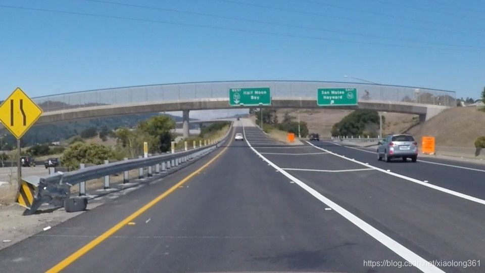
下图是一张安装在汽车上的前向相机在道路上拍摄下的图像。
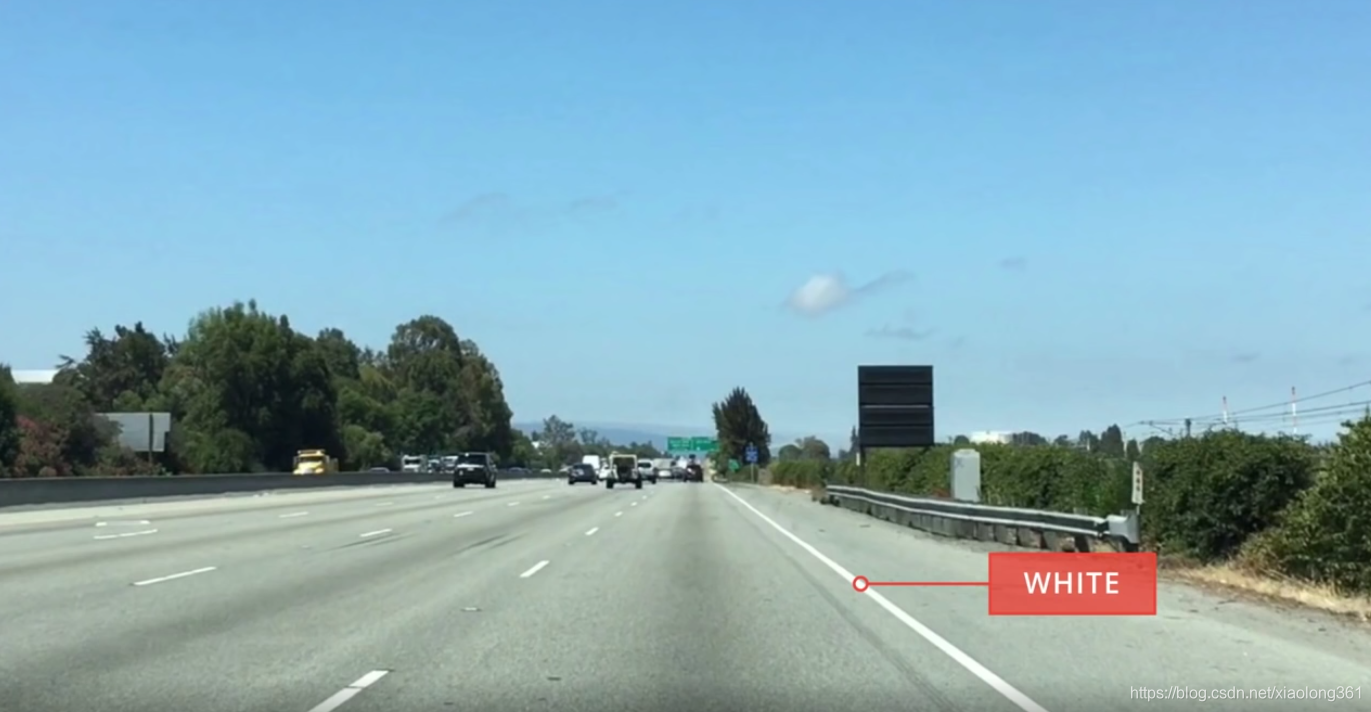
从图像中可以看出,车道线的颜色信息是可以将它和周围环境区分开来的明显特征。因此我们首先来学习如何通过颜色选择对图像上的车道线相关信息进行提取。
如下图所示,对于彩色相机拍摄得到的图像,我们可以将其按下图所示分成三个颜色通道(三基色):红(R)、绿(G)、蓝(B)。
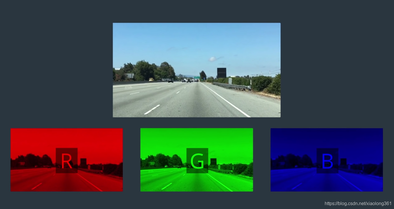
图像中的每个颜色通道相互独立,其每个像素中的值可以为[0,255]。当像素值为0时,对应的像素呈现黑色;当像素值为255时,对应的像素呈现该通道对应的颜色,如下图所示:
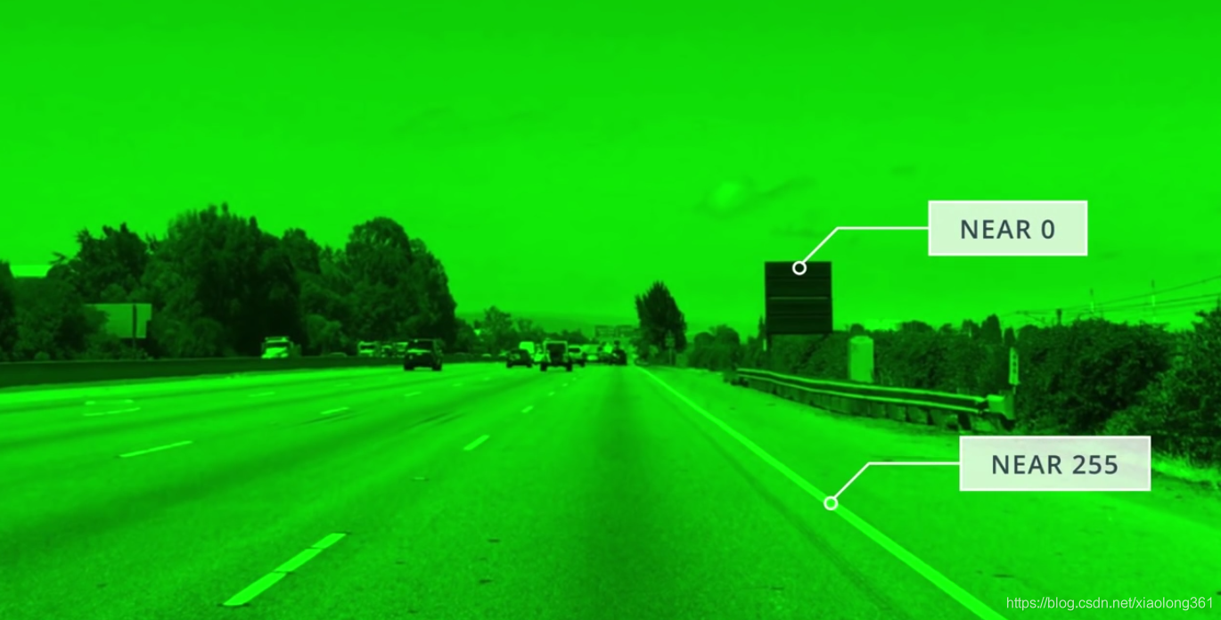
由上面的知识可知,如果我们用 [R,G,B] 的顺序表示像素值,则 [0,0,0] 对应像素的黑色,而 [255,255,255] 对应像素的白色。关于更多的颜色组合,若感兴趣可以通过网络上的在线颜色选择器工具进行查询。
代码实践
下面我们将通过Python编程实现简单的颜色选择。
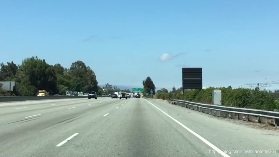
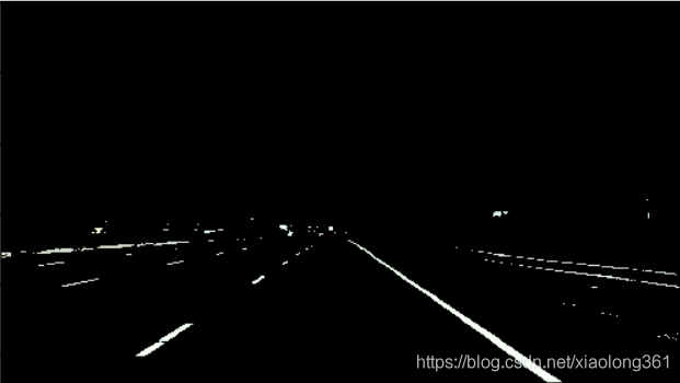
我们将对上面提到的相机图像进行处理,原始图像如下(如需测试程序,可在浏览器中保存到本地):
Python代码如下:
# -*- coding: utf-8 -*-#导入依赖库import matplotlib.pyplot as pltimport matplotlib.image as mpimgimport numpy as np# 利用matplotlib.image读取图片数据,并打印出图像的数据类型和数据维度image = mpimg.imread('test.jpg')print('This image is: ',type(image), # 将会输出 'with dimensions:', image.shape)# 将会输出(540, 960, 3)# Grab the x and y size and make a copy of the imageysize = image.shape[0] # image heightxsize = image.shape[1] # image width# Note: always make a copy rather than simply using "="color_select = np.copy(image)# Define our color selection criteriared_threshold = 200green_threshold = 200blue_threshold = 200# 利用上述三个阈值生成rgb_threshold阈值 。rgb_threshold = [red_threshold, green_threshold, blue_threshold]# 选出小于阈值的像素并将它们的值置为0(黑色),对大于等于阈值的像素进行保留.# Identify pixels below the thresholdthresholds = (image[:,:,0] < rgb_threshold[0]) \ | (image[:,:,1] < rgb_threshold[1]) \ | (image[:,:,2] < rgb_threshold[2])color_select[thresholds] = [0,0,0] # to black# Display the image plt.imshow(color_select)plt.show()# Uncomment the following code if you are running the code locally and wish to save the image# mpimg.imsave("test-after.png", color_select)最终,程序会将图像中小于阈值的像素全部置为黑色,仅保留大于等于阈值的像素值。
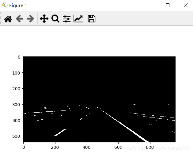
程序运行结果如下,由结果可知,我们通过颜色选择去除了图像中大部分和车道线无关的信息:
区域筛选(Region Masking)
理论基础
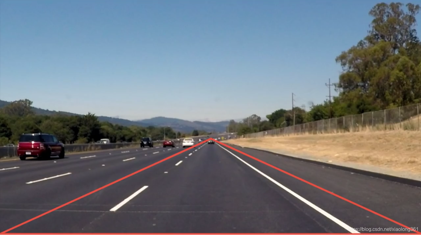
上一节我们通过简单的颜色选择得到了上图所示的包含车道线的像素信息,下面需要进一步提取出当前车辆所在的车道线信息。我们暂时假设相机位于车辆正中,且相机视角中心处于车辆正前方,且当前车道为直线车道。因此对于当前车道线提取,我们感兴趣的图像区域如下图红色区域所示:
 下面我们需要将感兴趣区域筛选与颜色选择结合起来,对经过颜色选择得到的像素信息进行区域筛选,并将符合条件的像素置为红色,即可得到当前车道的车道线信息,具体代码实现见下一节。
代码实践
Python代码如下:
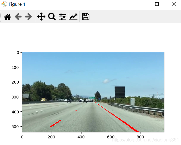
# -*- coding: utf-8 -*-#导入依赖库import matplotlib.pyplot as pltimport matplotlib.image as mpimgimport numpy as np# 利用matplotlib.image读取图片数据,并打印出图像的数据类型和数据维度image = mpimg.imread('test.jpg')print('This image is: ',type(image), # 将会输出 'with dimensions:', image.shape)# 将会输出(540, 960, 3)# Grab the x and y size and make a copy of the imageysize = image.shape[0] # image heightxsize = image.shape[1] # image width# Note: always make a copy rather than simply using "="color_select = np.copy(image)line_image = np.copy(image)# Define our color selection criteriared_threshold = 200green_threshold = 200blue_threshold = 200# 利用上述三个阈值生成rgb_threshold阈值 。rgb_threshold = [red_threshold, green_threshold, blue_threshold]# Define a triangle region of interest (Note: if you run this code, # Keep in mind the origin (x=0, y=0) is in the upper left in image processingleft_bottom = [0, 539] #三角区域的左下角right_bottom = [900, 539] #三角区域的右下角apex = [475, 320] #三角区域的顶点# 利用polyfit函数根据直线的两个端点得到连线,输入参数“1”表示曲线最高阶数为1(直线)# 得到直线 ax+b 的参数 a和bfit_left = np.polyfit((left_bottom[0], apex[0]), (left_bottom[1], apex[1]), 1)fit_right = np.polyfit((right_bottom[0], apex[0]), (right_bottom[1], apex[1]), 1)fit_bottom = np.polyfit((left_bottom[0], right_bottom[0]), (left_bottom[1], right_bottom[1]), 1)# 选出低于阈值的像素并将它们的值置为0(黑色),对高于阈值的像素进行保留.# Identify pixels below the thresholdcolor_thresholds = (image[:,:,0] < rgb_threshold[0]) \ | (image[:,:,1] < rgb_threshold[1]) \ | (image[:,:,2] < rgb_threshold[2])color_select[color_thresholds] = [0,0,0] # to black# Find the region inside the linesXX, YY = np.meshgrid(np.arange(0, xsize), np.arange(0, ysize))region_thresholds = (YY > (XX*fit_left[0] + fit_left[1])) & \ (YY > (XX*fit_right[0] + fit_right[1])) & \ (YY < (XX*fit_bottom[0] + fit_bottom[1]))# Find where image is both colored right and in the region# 将原图中大于等于颜色选择阈值且位于感兴趣区域中的像素设置为红色。line_image[~color_thresholds & region_thresholds] = [255,0,0]# Display our two output images(重合显示)#plt.imshow(color_select)plt.imshow(line_image)plt.show()程序运行结果如下图所示:
Canny边缘检测
问题背景
基于颜色选择原理来提取单一颜色(如白色)的车道线对于自动驾驶来说是远远不够的,因为车道线不是只有一种颜色,而且即使是同一颜色的车道线也可能会因为不同的光线条件(如白天、夜晚)而具有不同的颜色,从而导致检测失败。
为了让我们的算法可以提取任意颜色的车道线,我们需要引入复杂的计算机视觉方法。
后面的课程我们将详细介绍一些计算机视觉技术,并且让你直观地认识到它们是如何工作的。我们会利用OpenCV使用这些算法,并进一步实现车道线提取功能。关于计算机视觉技术的全面讲解,请参考优达学城的免费课程:Introduction to Computer Vision。

在本课程中,我们将使用Python版本的OpenCV完成计算机视觉算法相关的工作。OpenCV表示“Open-Source Computer Vision”,即开源的计算机视觉。OpenCV包含了大量的计算机视觉算法函数库可供使用,关于其详细介绍请移步OpenCV官网。
要安装Python下的OpenCV可以在命令行利用如下命令通过清华镜像源下载安装:
pip install opencv-python -i https://pypi.tuna.tsinghua.edu.cn/simple
本节中我们要讲的计算机视觉算法是Canny边缘检测。
Canny边缘检测原理
简单来说,Canndy边缘检测的算法原理是:
- 首先我们需要将彩色图像转换为灰度图像,也就是将彩色图像的三个通道转换为一个通道,每个像素对应一个0到255的整数值用于表示灰度大小。
- 然后利用高斯滤波器对图像进行高斯模糊去噪(关于高斯模糊,可以参考OpenCV gaussianblur文档)。
- 随后对去噪后的灰度图计算梯度(gradient),得到图像中每个像素点对应的强度梯度。梯度值代表了该像素点与周围像素值的变化关系,变化越大则梯度值越大。一般来说,在图像中物体的边缘通常会表现出较大的梯度值。
- Canny算法可以从梯度图像中提取出像素梯度大小处于一定范围的边界点集合,并针对较粗的边缘,利用非极大值抑制算法,过滤掉边缘附近的部分像素,从而只保留图像中位于实际边缘的较细的边缘线。
关于OpenCV中Canny算法的详细原理说明,请参考OpenCV Canny 文档。
我们即将使用的OpenCV的Canny算法函数接口定义如下:
edges=cv2.Canny(image, low_threshold, high_threshold)
该函数能够利用Canny算法检测输入图像image中的边缘,并将它们标记在输出图像edges中,edges与image具有相同的尺寸。
关于2个阈值参数:
- 低于阈值
low_threshold的像素点会被认为不是边缘。 - 高于阈值
high_threshold的像素点会被认为是边缘。 - 在阈值
low_threshold和阈值high_threshold之间的像素点,若与第2步得到的边缘像素点相邻,则被认为是边缘,否则被认为不是边缘。
注意:在OpenCV Canny 文档中,建议阈值
low_threshold和阈值high_threshold的比率在1:2和1:3之间。
关于该函数的完整接口说明,请参考OpenCV API文档。
代码实践
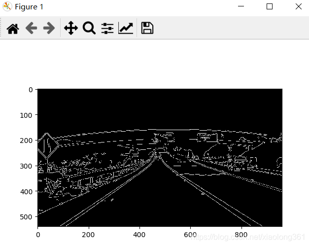
下面我们将利用下面这幅图像展示如何利用Canny算法对图像进行边缘检测。
Python代码如下:
# -*- coding: utf-8 -*-#导入依赖库import matplotlib.pyplot as pltimport matplotlib.image as mpimgimport numpy as npimport cv2# Read in the image and convert to grayscaleimage = mpimg.imread('exit-ramp.jpg')gray = cv2.cvtColor(image, cv2.COLOR_RGB2GRAY)# Define a kernel size for Gaussian smoothing / blurring# Note: this step is optional as cv2.Canny() applies a 5x5 Gaussian internallykernel_size = 5blur_gray = cv2.GaussianBlur(gray,(kernel_size, kernel_size), 0)# Define parameters for Canny and run itlow_threshold = 50high_threshold = 150edges = cv2.Canny(blur_gray, low_threshold, high_threshold)# Display the imageplt.imshow(edges, cmap='Greys_r')程序运行得到的边缘检测结果如下:
霍夫变换(Hough Transform)
本节我们将学习如何利用霍夫变换从Canny边缘中找到车道线。
目前我们已经得到了Canny算法检测到的边缘点,我们需要用一种方法将这些点中呈现为直线的车道线找出来,这可以通过霍夫变换来实现。
理论基础
霍夫变换的算法流程大致如下:给定一个物件、要辨别的形状的种类,算法会在参数空间(parameter space)中执行投票来决定物体的形状,而这是由累加空间(accumulator space)里的局部最大值(local maximum)来决定。关于霍夫变换的详细说明,请参考霍夫变换-百度百科。
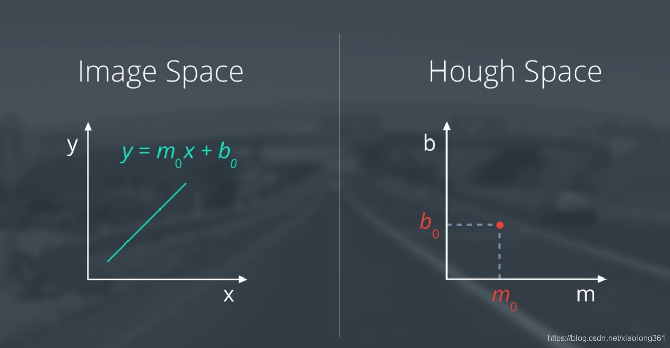
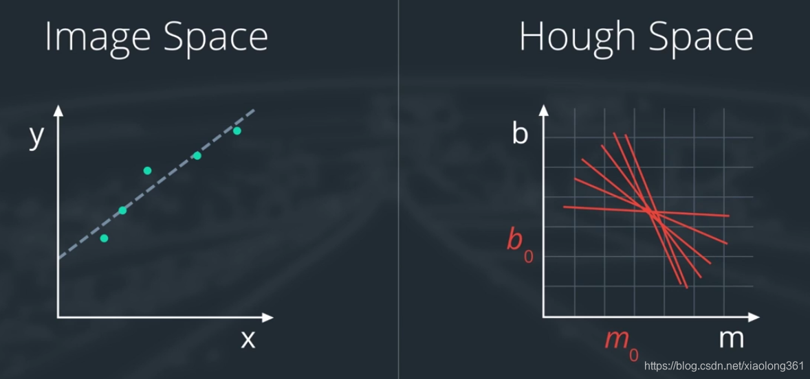
对于我们需要解决的车道线问题,在图像空间(Image Space)中我们可以将其视为直线,形式为:
y =m0 x +b0 y=m_0 x+b_0 y=m0x+b0
而在对应的霍夫空间(Hough Space,也可以简单将其理解为“参数空间”)中,相应的直线可以直接用 m 0 m_0 m0和 b 0 b_0 b0的组合来表示。于是经过霍夫变换,图像空间中的一条直线将被转换为霍夫空间中的一个点,如下图所示。
同理,有:
- 图像空间中的点( x , y ) (x,y) (x,y)对应霍夫空间下的直线b = y − x m b=y-xm b=y−xm。
- 霍夫空间下的两条直线的交点对应图像空间中的一条直线,该直线上存在两个点分别与霍夫空间中的两条直线对应。
- 图像空间中的一条直线的多个点,对应霍夫空间中的多条直线相交于一点,示意图如下。
我们知道,Canny边缘检测得到的结果是图像中所有被视为边缘的点,这些点也就对应于霍夫空间中的多条直线。要想提取出图像空间中处于同一直线上的点,也就是需要找到霍夫空间中相交于一点的直线。
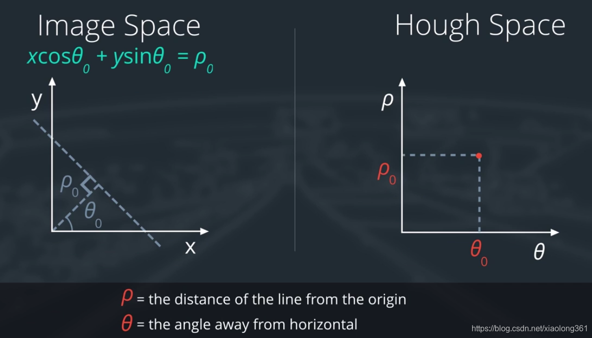
由于用 y = m x + b y=m x+b y=mx+b的形式表示直线,会存在平行于y轴的直线斜率为无穷的情况,因此我们采用“sine Hough”空间用来避免这一问题。在图像空间中,我们用 ρ \rho ρ来表示直线到原点的距离,用 θ \theta θ表示从x轴到直线垂线的角度,具体表示形式如下图所示。即在霍夫空间用参数 ( θ , ρ ) (\theta,\rho) (θ,ρ)来代替参数 ( m , b ) (m,b) (m,b)。
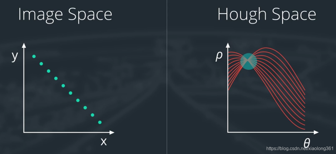
基于此,图像空间中的一点将对应“sine Hough”空间下的一条正弦曲线,如下图所示:
代码实践
我们利用OpenCV中的函数HoughLinesP来提取Canny边缘检测结果中的直线。要学习如何从头编写霍夫变换的代码,可以参考网站Understanding Hough Transform With Python。
让我们先来看一下OpenCV中函数HoughLinesP的声明:
lines = cv2.HoughLinesP(masked_edges, rho, theta, threshold, np.array([]), min_line_length, max_line_gap)其中,masked_edges是输入的边缘图像(来自Canny算法输出),该函数的输出lines是包含线段起始点信息(x1,y1,x2,y2)的数组。其他参数定义了我们需要的是什么样的线段。
首先,rho和theta分别表示霍夫变换算法中栅格的距离和角度分辨率。需要注意的是,在霍夫空间中的 ( θ , ρ ) (\theta,\rho) (θ,ρ)坐标系中定义了栅格,用来近似化求解空间中曲线的交点等信息,rho的单位应为像素,最小值为1;theta的单位应为弧度,初始值通常可设置为1度(pi/180 rad)。
threshold参数指定算法中投票的最小值(即给定栅格中的曲线交点个数),只有当某个栅格中的曲线交点个数大于threshold时,才认为其是一条应该输出的线段。
参数中的np.array([])只是一个placeholder,使用时无需修改。参数min_line_length是一条输出线段的最小长度(单位为像素),参数max_line_gap是连接两个独立线段成为一条输出线段的最大线段间隔(单位为像素)。
另外,前面的课程中我们曾手写过一个图像中的三角形区域筛选算法,这一次我们可以用OpenCV的cv2.fillPoly()函数来实现对四边形区域的筛选(该函数其实可以实现对任意复杂的多边形区域进行筛选),具体用法参考下面的代码。
下面是Python代码,程序执行流程主要包括:
加载图像->灰度转换->高斯模糊->Canny边缘检测->fillPoly目标区域筛选->HoughLinesP直线提取->结果可视化。
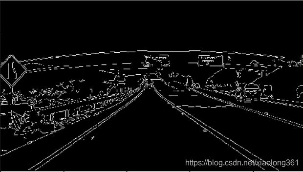
# -*- coding: utf-8 -*-#导入依赖库import matplotlib.pyplot as pltimport matplotlib.image as mpimgimport numpy as npimport cv2# Read in and grayscale the imageimage = mpimg.imread('exit-ramp.jpg')gray = cv2.cvtColor(image,cv2.COLOR_RGB2GRAY)# Define a kernel size and apply Gaussian smoothingkernel_size = 5blur_gray = cv2.GaussianBlur(gray,(kernel_size, kernel_size),0)# Define our parameters for Canny and applylow_threshold = 50high_threshold = 150edges = cv2.Canny(blur_gray, low_threshold, high_threshold)# Next we'll create a masked edges image using cv2.fillPoly()mask = np.zeros_like(edges) ignore_mask_color = 255 # This time we are defining a four sided polygon to maskimshape = image.shape#vertices = np.array([[(0,imshape[0]),(0, 0), (imshape[1], 0), (imshape[1],imshape[0])]], dtype=np.int32)vertices = np.array([[(0,imshape[0]),(450, 290), (490, 290), (imshape[1],imshape[0])]], dtype=np.int32)cv2.fillPoly(mask, vertices, ignore_mask_color)masked_edges = cv2.bitwise_and(edges, mask)# Define the Hough transform parameters# Make a blank the same size as our image to draw onrho = 2 # distance resolution in pixels of the Hough gridtheta = np.pi/180 # angular resolution in radians of the Hough gridthreshold = 15 # minimum number of votes (intersections in Hough grid cell)min_line_length = 30 #minimum number of pixels making up a linemax_line_gap = 20 # maximum gap in pixels between connectable line segmentsline_image = np.copy(image)*0 # creating a blank to draw lines on# Run Hough on edge detected image# Output "lines" is an array containing endpoints of detected line segmentslines = cv2.HoughLinesP(masked_edges, rho, theta, threshold, np.array([]),min_line_length, max_line_gap)# Iterate over the output "lines" and draw lines on a blank image,for line in lines: for x1,y1,x2,y2 in line: cv2.line(line_image,(x1,y1),(x2,y2),(255,0,0),10)# Create a "color" binary image to combine with line image(因为line_image为RGB图像)color_edges = np.dstack((edges, edges, edges)) # Draw the lines on the edge image。其中,color_edges不透明度0.8,line_image不透明度1.lines_edges = cv2.addWeighted(color_edges, 0.8, line_image, 1, 0) plt.imshow(lines_edges)plt.show()程序运行后得到的车道线提取结果如下:
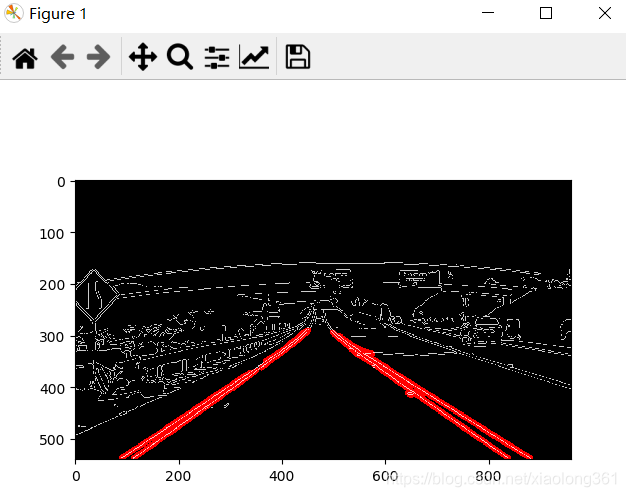
由结果可以看到,我们通过选取合适的算法参数,从图像中提取出了当前车道的车道线信息。