【机器学习】使用scikit-learn实现多项式回归(10min阅读时长)
Polynomial Regression(多项式回归)
Objectives(目标)
看完这篇文章,将会:1.使用scikit-learn实现多项式回归 2.创建一个模型,训练它,测试它,并使用它
After completing this lab you will be able to:
- Use scikit-learn to implement Polynomial Regression
- Create a model, train it, test it and use the model
Table of contents
- Downloading Data(下载数据)
- Polynomial regression(进行多项式回归)
- Evaluation(评估)
- Practice(进一步练习)
Importing Needed packages(导入相关库)
import matplotlib.pyplot as pltimport pandas as pdimport pylab as plimport numpy as np%matplotlib inlineDownloading Data(下载数据)
FuelConsumption(点我下载)
Understanding the Data(理解数据)
FuelConsumption.csv:
我们下载了一个油耗数据集, FuelConsumption.csv,其中包含了加拿大零售新轻型汽车的特定车型油耗等级和估计的二氧化碳排放量。
We have downloaded a fuel consumption dataset, FuelConsumption.csv, which contains model-specific fuel consumption ratings and estimated carbon dioxide emissions for new light-duty vehicles for retail sale in Canada. Dataset source
- MODELYEAR e.g. 2014
- MAKE e.g. Acura
- MODEL e.g. ILX
- VEHICLE CLASS e.g. SUV
- ENGINE SIZE e.g. 4.7
- CYLINDERS e.g 6
- TRANSMISSION e.g. A6
- FUELTYPE e.g. z
- FUEL CONSUMPTION in CITY(L/100 km) e.g. 9.9
- FUEL CONSUMPTION in HWY (L/100 km) e.g. 8.9
- FUEL CONSUMPTION COMB (L/100 km) e.g. 9.2
- CO2 EMISSIONS (g/km) e.g. 182 --> low --> 0
Reading the data in(读取数据)
# df = pd.read_csv("FuelConsumption.csv")df=pd.read_csv("D:\MLwithPython\FuelConsumptionCo2.csv")# take a look at the datasetdf.head()| MODELYEAR | MAKE | MODEL | VEHICLECLASS | ENGINESIZE | CYLINDERS | TRANSMISSION | FUELTYPE | FUELCONSUMPTION_CITY | FUELCONSUMPTION_HWY | FUELCONSUMPTION_COMB | FUELCONSUMPTION_COMB_MPG | CO2EMISSIONS | |
|---|---|---|---|---|---|---|---|---|---|---|---|---|---|
| 0 | 2014 | ACURA | ILX | COMPACT | 2.0 | 4 | AS5 | Z | 9.9 | 6.7 | 8.5 | 33 | 196 |
| 1 | 2014 | ACURA | ILX | COMPACT | 2.4 | 4 | M6 | Z | 11.2 | 7.7 | 9.6 | 29 | 221 |
| 2 | 2014 | ACURA | ILX HYBRID | COMPACT | 1.5 | 4 | AV7 | Z | 6.0 | 5.8 | 5.9 | 48 | 136 |
| 3 | 2014 | ACURA | MDX 4WD | SUV - SMALL | 3.5 | 6 | AS6 | Z | 12.7 | 9.1 | 11.1 | 25 | 255 |
| 4 | 2014 | ACURA | RDX AWD | SUV - SMALL | 3.5 | 6 | AS6 | Z | 12.1 | 8.7 | 10.6 | 27 | 244 |
Let’s select some features that we want to use for regression.
cdf = df[['ENGINESIZE','CYLINDERS','FUELCONSUMPTION_COMB','CO2EMISSIONS']]cdf.head(9)| ENGINESIZE | CYLINDERS | FUELCONSUMPTION_COMB | CO2EMISSIONS | |
|---|---|---|---|---|
| 0 | 2.0 | 4 | 8.5 | 196 |
| 1 | 2.4 | 4 | 9.6 | 221 |
| 2 | 1.5 | 4 | 5.9 | 136 |
| 3 | 3.5 | 6 | 11.1 | 255 |
| 4 | 3.5 | 6 | 10.6 | 244 |
| 5 | 3.5 | 6 | 10.0 | 230 |
| 6 | 3.5 | 6 | 10.1 | 232 |
| 7 | 3.7 | 6 | 11.1 | 255 |
| 8 | 3.7 | 6 | 11.6 | 267 |
让我们来画一下排放量和引擎大小的关系吧
Let’s plot Emission values with respect to Engine size:
plt.scatter(cdf.ENGINESIZE, cdf.CO2EMISSIONS, color='blue')plt.xlabel("Engine size")plt.ylabel("Emission")plt.show()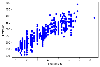
Creating train and test dataset(创建训练集和测试集)
训练/测试分割涉及将数据集分割为互斥的训练集和测试集。 之后,使用训练集进行训练,使用测试集进行测试。
Train/Test Split involves splitting the dataset into training and testing sets respectively, which are mutually exclusive. After which, you train with the training set and test with the testing set.
msk = np.random.rand(len(df)) < 0.8train = cdf[msk]test = cdf[~msk]Polynomial regression(多项式回归)
有时候,数据的趋势不是线性的,而是一个曲线。在这种情况下,我们就使用多项式回归的方法。多项式回归可以用来拟合一次、二次、三次等等的数据。
Sometimes, the trend of data is not really linear, and looks curvy. In this case we can use Polynomial regression methods. In fact, many different regressions exist that can be used to fit whatever the dataset looks like, such as quadratic, cubic, and so on, and it can go on and on to infinite degrees.
实际上就是建立一个y关于x的n次多项式的一个函数,下面就是以2次为例。
In essence, we can call all of these, polynomial regression, where the relationship between the independent variable x and the dependent variable y is modeled as an nth degree polynomial in x. Lets say you want to have a polynomial regression (let’s make 2 degree polynomial):
y = b + θ _ 1 x + θ _ 2x2 y = b + \theta\_{1} x + \theta\_{2} x^2 y=b+θ_1x+θ_2x2
现在的问题就是:我们只有x的一次项而没有其他次数项。
Now, the question is: how we can fit our data on this equation while we have only x values, such as Engine Size?
那我们就创建这几个特征: 1, x x x, and x 2 x^2 x2。
Well, we can create a few additional features: 1, x x x, and x 2 x^2 x2.
要完成这个操作,我们用到sklearn的PolynomialFeatures() 函数。具体方法见下面代码。
PolynomialFeatures() function in Scikit-learn library, drives a new feature sets from the original feature set. That is, a matrix will be generated consisting of all polynomial combinations of the features with degree less than or equal to the specified degree. For example, lets say the original feature set has only one feature, ENGINESIZE. Now, if we select the degree of the polynomial to be 2, then it generates 3 features, degree=0, degree=1 and degree=2:
from sklearn.preprocessing import PolynomialFeaturesfrom sklearn import linear_modeltrain_x = np.asanyarray(train[['ENGINESIZE']])train_y = np.asanyarray(train[['CO2EMISSIONS']])test_x = np.asanyarray(test[['ENGINESIZE']])test_y = np.asanyarray(test[['CO2EMISSIONS']])poly = PolynomialFeatures(degree=2)train_x_poly = poly.fit_transform(train_x)# print(train_x)print(train_x_poly)# 可以看到第一列是相当于零次方,第二列是一次方,第三列就是二次方[[ 1. 2. 4. ] [ 1. 2.4 5.76] [ 1. 1.5 2.25] ... [ 1. 3. 9. ] [ 1. 3.2 10.24] [ 1. 3.2 10.24]]fit_transform takes our x values, and output a list of our data raised from power of 0 to power of 2 (since we set the degree of our polynomial to 2).
The equation and the sample example is displayed below.
这是不是看上去就像是多元线性回归一样了呢,没错,就是这样的。之前写的多元线性回归的博客
It looks like feature sets for multiple linear regression analysis, right? Yes. It Does.
Indeed, Polynomial regression is a special case of linear regression, with the main idea of how do you select your features. Just consider replacing the x x x with x _ 1 x\_1 x_1, x _ 1 2 x\_1^2 x_12 with x _ 2 x\_2 x_2, and so on. Then the 2nd degree equation would be turn into:
y = b + θ _ 1 x _ 1 + θ _ 2 x _ 2 y = b + \theta\_1 x\_1 + \theta\_2 x\_2 y=b+θ_1x_1+θ_2x_2
现在,我们可以把它当作一个“线性回归”问题来处理。 因此,该多项式回归被认为是传统多元线性回归的特例。 所以,你可以用线性回归的相同机制来解决这些问题。
Now, we can deal with it as a ‘linear regression’ problem. Therefore, this polynomial regression is considered to be a special case of traditional multiple linear regression. So, you can use the same mechanism as linear regression to solve such problems.
所以,我们就用之前就用过的 LinearRegression()函数来解决。
so we can use LinearRegression() function to solve it:
clf = linear_model.LinearRegression()train_y_ = clf.fit(train_x_poly, train_y)# The coefficientsprint ('Coefficients: ', clf.coef_)print ('Intercept: ',clf.intercept_)Coefficients: [[ 0. 47.51814244 -1.13641106]]Intercept: [112.0368771]如前所述,系数和截距是拟合曲线的参数。
这是多元线性回归,有3个参数,这些参数是截距和系数,sklearn从我们的新特征集中估计了它们。 我们来画一下吧:
As mentioned before, Coefficient and Intercept , are the parameters of the fit curvy line.
Given that it is a typical multiple linear regression, with 3 parameters, and knowing that the parameters are the intercept and coefficients of hyperplane, sklearn has estimated them from our new set of feature sets. Lets plot it:
plt.scatter(train.ENGINESIZE, train.CO2EMISSIONS, color='blue')XX = np.arange(0.0, 10.0, 0.1)print(XX)yy = clf.intercept_[0]+ clf.coef_[0][1]*XX+ clf.coef_[0][2]*np.power(XX, 2)plt.plot(XX, yy, '-r' )plt.xlabel("Engine size")plt.ylabel("Emission")[0. 0.1 0.2 0.3 0.4 0.5 0.6 0.7 0.8 0.9 1. 1.1 1.2 1.3 1.4 1.5 1.6 1.7 1.8 1.9 2. 2.1 2.2 2.3 2.4 2.5 2.6 2.7 2.8 2.9 3. 3.1 3.2 3.3 3.4 3.5 3.6 3.7 3.8 3.9 4. 4.1 4.2 4.3 4.4 4.5 4.6 4.7 4.8 4.9 5. 5.1 5.2 5.3 5.4 5.5 5.6 5.7 5.8 5.9 6. 6.1 6.2 6.3 6.4 6.5 6.6 6.7 6.8 6.9 7. 7.1 7.2 7.3 7.4 7.5 7.6 7.7 7.8 7.9 8. 8.1 8.2 8.3 8.4 8.5 8.6 8.7 8.8 8.9 9. 9.1 9.2 9.3 9.4 9.5 9.6 9.7 9.8 9.9]Text(0, 0.5, 'Emission')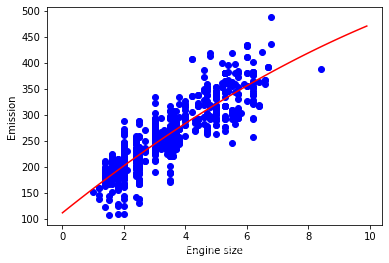
Evaluation(评估)
from sklearn.metrics import r2_scoretest_x_poly = poly.transform(test_x)test_y_ = clf.predict(test_x_poly)print("Mean absolute error: %.2f" % np.mean(np.absolute(test_y_ - test_y)))print("Residual sum of squares (MSE): %.2f" % np.mean((test_y_ - test_y) 2))print("R2-score: %.2f" % r2_score(test_y,test_y_ ) )Mean absolute error: 23.68Residual sum of squares (MSE): 983.44R2-score: 0.77Practice(进一步练习)
前面用的是二次拟合,现在我们试试三次拟合吧!准确性会更好吗? Try to use a polynomial regression with the dataset but this time with degree three (cubic). Does it result in better accuracy?
# write your code herefrom sklearn.preprocessing import PolynomialFeaturesfrom sklearn import linear_modeltrain_x = np.asanyarray(train[['ENGINESIZE']])train_y = np.asanyarray(train[['CO2EMISSIONS']])test_x = np.asanyarray(test[['ENGINESIZE']])test_y = np.asanyarray(test[['CO2EMISSIONS']])poly = PolynomialFeatures(degree=3)train_x_poly = poly.fit_transform(train_x)# print(train_x)print(train_x_poly)# 可以看到第一列是相当于零次方,第二列是一次方,第三列就是二次方,第四列是三次方clf = linear_model.LinearRegression()train_y_ = clf.fit(train_x_poly, train_y)# The coefficientsprint ('Coefficients: ', clf.coef_)print ('Intercept: ',clf.intercept_)plt.scatter(train.ENGINESIZE, train.CO2EMISSIONS, color='blue')XX = np.arange(0.0, 10.0, 0.1)print(XX)yy = clf.intercept_[0]+ clf.coef_[0][1]*XX+ clf.coef_[0][2]*np.power(XX, 2)+ clf.coef_[0][3]*np.power(XX, 3)plt.plot(XX, yy, '-r' )plt.xlabel("Engine size")plt.ylabel("Emission")from sklearn.metrics import r2_scoretest_x_poly = poly.transform(test_x)test_y_ = clf.predict(test_x_poly)print("Mean absolute error: %.2f" % np.mean(np.absolute(test_y_ - test_y)))print("Residual sum of squares (MSE): %.2f" % np.mean((test_y_ - test_y) 2))print("R2-score: %.2f" % r2_score(test_y,test_y_ ) )[[ 1. 2. 4. 8. ] [ 1. 2.4 5.76 13.824] [ 1. 1.5 2.25 3.375] ... [ 1. 3. 9. 27. ] [ 1. 3.2 10.24 32.768] [ 1. 3.2 10.24 32.768]]Coefficients: [[ 0. 30.21883468 3.69813705 -0.40815132]]Intercept: [130.27379894][0. 0.1 0.2 0.3 0.4 0.5 0.6 0.7 0.8 0.9 1. 1.1 1.2 1.3 1.4 1.5 1.6 1.7 1.8 1.9 2. 2.1 2.2 2.3 2.4 2.5 2.6 2.7 2.8 2.9 3. 3.1 3.2 3.3 3.4 3.5 3.6 3.7 3.8 3.9 4. 4.1 4.2 4.3 4.4 4.5 4.6 4.7 4.8 4.9 5. 5.1 5.2 5.3 5.4 5.5 5.6 5.7 5.8 5.9 6. 6.1 6.2 6.3 6.4 6.5 6.6 6.7 6.8 6.9 7. 7.1 7.2 7.3 7.4 7.5 7.6 7.7 7.8 7.9 8. 8.1 8.2 8.3 8.4 8.5 8.6 8.7 8.8 8.9 9. 9.1 9.2 9.3 9.4 9.5 9.6 9.7 9.8 9.9]Mean absolute error: 23.62Residual sum of squares (MSE): 972.79R2-score: 0.78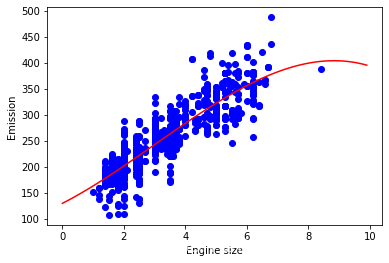
可以看到 R 2 R^2 R2确实大了一点,但也只大了0.01。