PyTorch学习笔记(七):PyTorch可视化
1 可视化网络结构
- 打印模型基础信息:使用
print()函数,只能打印出基础构件的信息,不能显示每一层的shape和对应参数量的大小
import torchvision.models as modelsmodel = models.resnet18()print(model)ResNet( (conv1): Conv2d(3, 64, kernel_size=(7, 7), stride=(2, 2), padding=(3, 3), bias=False) (bn1): BatchNorm2d(64, eps=1e-05, momentum=0.1, affine=True, track_running_stats=True) (relu): ReLU(inplace=True) (maxpool): MaxPool2d(kernel_size=3, stride=2, padding=1, dilation=1, ceil_mode=False) (layer1): Sequential( (0): BasicBlock( (conv1): Conv2d(64, 64, kernel_size=(3, 3), stride=(1, 1), padding=(1, 1), bias=False) (bn1): BatchNorm2d(64, eps=1e-05, momentum=0.1, affine=True, track_running_stats=True) (relu): ReLU(inplace=True) (conv2): Conv2d(64, 64, kernel_size=(3, 3), stride=(1, 1), padding=(1, 1), bias=False) (bn2): BatchNorm2d(64, eps=1e-05, momentum=0.1, affine=True, track_running_stats=True) ) (1): BasicBlock( (conv1): Conv2d(64, 64, kernel_size=(3, 3), stride=(1, 1), padding=(1, 1), bias=False) (bn1): BatchNorm2d(64, eps=1e-05, momentum=0.1, affine=True, track_running_stats=True) (relu): ReLU(inplace=True) (conv2): Conv2d(64, 64, kernel_size=(3, 3), stride=(1, 1), padding=(1, 1), bias=False) (bn2): BatchNorm2d(64, eps=1e-05, momentum=0.1, affine=True, track_running_stats=True) ) ) (layer2): Sequential( (0): BasicBlock( (conv1): Conv2d(64, 128, kernel_size=(3, 3), stride=(2, 2), padding=(1, 1), bias=False) (bn1): BatchNorm2d(128, eps=1e-05, momentum=0.1, affine=True, track_running_stats=True) (relu): ReLU(inplace=True) (conv2): Conv2d(128, 128, kernel_size=(3, 3), stride=(1, 1), padding=(1, 1), bias=False) (bn2): BatchNorm2d(128, eps=1e-05, momentum=0.1, affine=True, track_running_stats=True) (downsample): Sequential( (0): Conv2d(64, 128, kernel_size=(1, 1), stride=(2, 2), bias=False) (1): BatchNorm2d(128, eps=1e-05, momentum=0.1, affine=True, track_running_stats=True) ) ) (1): BasicBlock( (conv1): Conv2d(128, 128, kernel_size=(3, 3), stride=(1, 1), padding=(1, 1), bias=False) (bn1): BatchNorm2d(128, eps=1e-05, momentum=0.1, affine=True, track_running_stats=True) (relu): ReLU(inplace=True) (conv2): Conv2d(128, 128, kernel_size=(3, 3), stride=(1, 1), padding=(1, 1), bias=False) (bn2): BatchNorm2d(128, eps=1e-05, momentum=0.1, affine=True, track_running_stats=True) ) ) (layer3): Sequential( (0): BasicBlock( (conv1): Conv2d(128, 256, kernel_size=(3, 3), stride=(2, 2), padding=(1, 1), bias=False) (bn1): BatchNorm2d(256, eps=1e-05, momentum=0.1, affine=True, track_running_stats=True) (relu): ReLU(inplace=True) (conv2): Conv2d(256, 256, kernel_size=(3, 3), stride=(1, 1), padding=(1, 1), bias=False) (bn2): BatchNorm2d(256, eps=1e-05, momentum=0.1, affine=True, track_running_stats=True) (downsample): Sequential( (0): Conv2d(128, 256, kernel_size=(1, 1), stride=(2, 2), bias=False) (1): BatchNorm2d(256, eps=1e-05, momentum=0.1, affine=True, track_running_stats=True) ) ) (1): BasicBlock( (conv1): Conv2d(256, 256, kernel_size=(3, 3), stride=(1, 1), padding=(1, 1), bias=False) (bn1): BatchNorm2d(256, eps=1e-05, momentum=0.1, affine=True, track_running_stats=True) (relu): ReLU(inplace=True) (conv2): Conv2d(256, 256, kernel_size=(3, 3), stride=(1, 1), padding=(1, 1), bias=False) (bn2): BatchNorm2d(256, eps=1e-05, momentum=0.1, affine=True, track_running_stats=True) ) ) (layer4): Sequential( (0): BasicBlock( (conv1): Conv2d(256, 512, kernel_size=(3, 3), stride=(2, 2), padding=(1, 1), bias=False) (bn1): BatchNorm2d(512, eps=1e-05, momentum=0.1, affine=True, track_running_stats=True) (relu): ReLU(inplace=True) (conv2): Conv2d(512, 512, kernel_size=(3, 3), stride=(1, 1), padding=(1, 1), bias=False) (bn2): BatchNorm2d(512, eps=1e-05, momentum=0.1, affine=True, track_running_stats=True) (downsample): Sequential( (0): Conv2d(256, 512, kernel_size=(1, 1), stride=(2, 2), bias=False) (1): BatchNorm2d(512, eps=1e-05, momentum=0.1, affine=True, track_running_stats=True) ) ) (1): BasicBlock( (conv1): Conv2d(512, 512, kernel_size=(3, 3), stride=(1, 1), padding=(1, 1), bias=False) (bn1): BatchNorm2d(512, eps=1e-05, momentum=0.1, affine=True, track_running_stats=True) (relu): ReLU(inplace=True) (conv2): Conv2d(512, 512, kernel_size=(3, 3), stride=(1, 1), padding=(1, 1), bias=False) (bn2): BatchNorm2d(512, eps=1e-05, momentum=0.1, affine=True, track_running_stats=True) ) ) (avgpool): AdaptiveAvgPool2d(output_size=(1, 1)) (fc): Linear(in_features=512, out_features=1000, bias=True))- 可视化网络结构:使用
torchinfo库进行模型网络的结构输出,可以得到更加详细的信息,包括模块信息(每一层的类型、输出shape和参数量)、模型整体的参数量、模型大小、一次前向或者反向传播需要的内存大小等
import torchvision.models as modelsfrom torchinfo import summaryresnet18 = models.resnet18() # 实例化模型# 其中batch_size为1,图片的通道数为3,图片的高宽为224summary(model, (1, 3, 224, 224))==========================================================================================Layer (type:depth-idx) Output ShapeParam #==========================================================================================ResNet-- --├─Conv2d: 1-1[1, 64, 112, 112] 9,408├─BatchNorm2d: 1-2 [1, 64, 112, 112] 128├─ReLU: 1-3 [1, 64, 112, 112] --├─MaxPool2d: 1-4 [1, 64, 56, 56] --├─Sequential: 1-5 [1, 64, 56, 56] --│ └─BasicBlock: 2-1 [1, 64, 56, 56] --│ │ └─Conv2d: 3-1 [1, 64, 56, 56] 36,864│ │ └─BatchNorm2d: 3-2 [1, 64, 56, 56] 128│ │ └─ReLU: 3-3 [1, 64, 56, 56] --│ │ └─Conv2d: 3-4 [1, 64, 56, 56] 36,864│ │ └─BatchNorm2d: 3-5 [1, 64, 56, 56] 128│ │ └─ReLU: 3-6 [1, 64, 56, 56] --│ └─BasicBlock: 2-2 [1, 64, 56, 56] --│ │ └─Conv2d: 3-7 [1, 64, 56, 56] 36,864│ │ └─BatchNorm2d: 3-8 [1, 64, 56, 56] 128│ │ └─ReLU: 3-9 [1, 64, 56, 56] --│ │ └─Conv2d: 3-10 [1, 64, 56, 56] 36,864│ │ └─BatchNorm2d: 3-11 [1, 64, 56, 56] 128│ │ └─ReLU: 3-12 [1, 64, 56, 56] --├─Sequential: 1-6 [1, 128, 28, 28] --│ └─BasicBlock: 2-3 [1, 128, 28, 28] --│ │ └─Conv2d: 3-13 [1, 128, 28, 28] 73,728│ │ └─BatchNorm2d: 3-14 [1, 128, 28, 28] 256│ │ └─ReLU: 3-15 [1, 128, 28, 28] --│ │ └─Conv2d: 3-16 [1, 128, 28, 28] 147,456│ │ └─BatchNorm2d: 3-17 [1, 128, 28, 28] 256│ │ └─Sequential: 3-18 [1, 128, 28, 28] 8,448│ │ └─ReLU: 3-19 [1, 128, 28, 28] --│ └─BasicBlock: 2-4 [1, 128, 28, 28] --│ │ └─Conv2d: 3-20 [1, 128, 28, 28] 147,456│ │ └─BatchNorm2d: 3-21 [1, 128, 28, 28] 256│ │ └─ReLU: 3-22 [1, 128, 28, 28] --│ │ └─Conv2d: 3-23 [1, 128, 28, 28] 147,456│ │ └─BatchNorm2d: 3-24 [1, 128, 28, 28] 256│ │ └─ReLU: 3-25 [1, 128, 28, 28] --├─Sequential: 1-7 [1, 256, 14, 14] --│ └─BasicBlock: 2-5 [1, 256, 14, 14] --│ │ └─Conv2d: 3-26 [1, 256, 14, 14] 294,912│ │ └─BatchNorm2d: 3-27 [1, 256, 14, 14] 512│ │ └─ReLU: 3-28 [1, 256, 14, 14] --│ │ └─Conv2d: 3-29 [1, 256, 14, 14] 589,824│ │ └─BatchNorm2d: 3-30 [1, 256, 14, 14] 512│ │ └─Sequential: 3-31 [1, 256, 14, 14] 33,280│ │ └─ReLU: 3-32 [1, 256, 14, 14] --│ └─BasicBlock: 2-6 [1, 256, 14, 14] --│ │ └─Conv2d: 3-33 [1, 256, 14, 14] 589,824│ │ └─BatchNorm2d: 3-34 [1, 256, 14, 14] 512│ │ └─ReLU: 3-35 [1, 256, 14, 14] --│ │ └─Conv2d: 3-36 [1, 256, 14, 14] 589,824│ │ └─BatchNorm2d: 3-37 [1, 256, 14, 14] 512│ │ └─ReLU: 3-38 [1, 256, 14, 14] --├─Sequential: 1-8 [1, 512, 7, 7] --│ └─BasicBlock: 2-7 [1, 512, 7, 7] --│ │ └─Conv2d: 3-39 [1, 512, 7, 7] 1,179,648│ │ └─BatchNorm2d: 3-40 [1, 512, 7, 7] 1,024│ │ └─ReLU: 3-41 [1, 512, 7, 7] --│ │ └─Conv2d: 3-42 [1, 512, 7, 7] 2,359,296│ │ └─BatchNorm2d: 3-43 [1, 512, 7, 7] 1,024│ │ └─Sequential: 3-44 [1, 512, 7, 7] 132,096│ │ └─ReLU: 3-45 [1, 512, 7, 7] --│ └─BasicBlock: 2-8 [1, 512, 7, 7] --│ │ └─Conv2d: 3-46 [1, 512, 7, 7] 2,359,296│ │ └─BatchNorm2d: 3-47 [1, 512, 7, 7] 1,024│ │ └─ReLU: 3-48 [1, 512, 7, 7] --│ │ └─Conv2d: 3-49 [1, 512, 7, 7] 2,359,296│ │ └─BatchNorm2d: 3-50 [1, 512, 7, 7] 1,024│ │ └─ReLU: 3-51 [1, 512, 7, 7] --├─AdaptiveAvgPool2d: 1-9 [1, 512, 1, 1] --├─Linear: 1-10 [1, 1000] 513,000==========================================================================================Total params: 11,689,512Trainable params: 11,689,512Non-trainable params: 0Total mult-adds (G): 1.81==========================================================================================Input size (MB): 0.60Forward/backward pass size (MB): 39.75Params size (MB): 46.76Estimated Total Size (MB): 87.11==========================================================================================Copy to clipboardErrorCopied2 CNN可视化
- CNN卷积核可视化
model = models.vgg11(pretrained=True)dict(model.features.named_children()){'0': Conv2d(3, 64, kernel_size=(3, 3), stride=(1, 1), padding=(1, 1)), '1': ReLU(inplace=True), '2': MaxPool2d(kernel_size=2, stride=2, padding=0, dilation=1, ceil_mode=False), '3': Conv2d(64, 128, kernel_size=(3, 3), stride=(1, 1), padding=(1, 1)), '4': ReLU(inplace=True), '5': MaxPool2d(kernel_size=2, stride=2, padding=0, dilation=1, ceil_mode=False), '6': Conv2d(128, 256, kernel_size=(3, 3), stride=(1, 1), padding=(1, 1)), '7': ReLU(inplace=True), '8': Conv2d(256, 256, kernel_size=(3, 3), stride=(1, 1), padding=(1, 1)), '9': ReLU(inplace=True), '10': MaxPool2d(kernel_size=2, stride=2, padding=0, dilation=1, ceil_mode=False), '11': Conv2d(256, 512, kernel_size=(3, 3), stride=(1, 1), padding=(1, 1)), '12': ReLU(inplace=True), '13': Conv2d(512, 512, kernel_size=(3, 3), stride=(1, 1), padding=(1, 1)), '14': ReLU(inplace=True), '15': MaxPool2d(kernel_size=2, stride=2, padding=0, dilation=1, ceil_mode=False), '16': Conv2d(512, 512, kernel_size=(3, 3), stride=(1, 1), padding=(1, 1)), '17': ReLU(inplace=True), '18': Conv2d(512, 512, kernel_size=(3, 3), stride=(1, 1), padding=(1, 1)), '19': ReLU(inplace=True), '20': MaxPool2d(kernel_size=2, stride=2, padding=0, dilation=1, ceil_mode=False)}import matplotlib.pyplot as pltconv1 = dict(model.features.named_children())['3']# 得到第3层的卷积层参数kernel_set = conv1.weight.detach()num = len(conv1.weight.detach())print(kernel_set.shape)# 该代码仅可视化其中一个维度的卷积核,第3层的卷积核有128*64个for i in range(0, 1): i_kernel = kernel_set[i] plt.figure(figsize=(20, 17)) if (len(i_kernel)) > 1: for idx, filer in enumerate(i_kernel): plt.subplot(9, 9, idx+1) plt.axis('off') plt.imshow(filer[ :, :].detach(),cmap='bwr')torch.Size([128, 64, 3, 3])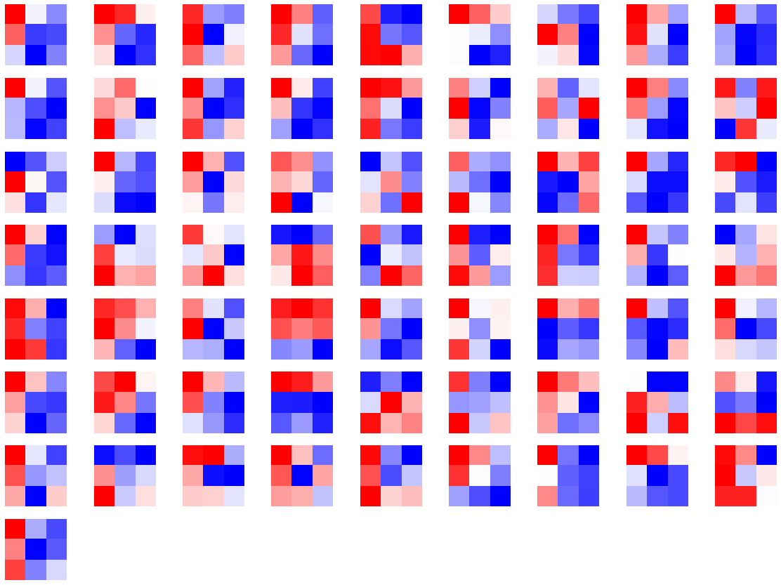
-
CNN特征图可视化:使用PyTorch提供的hook结构,得到网络在前向传播过程中的特征图。
-
CNN class activation map可视化:用于在CNN可视化场景下,判断图像中哪些像素点对预测结果是重要的,可使用
grad-cam库进行操作 -
使用FlashTorch快速实现CNDD可视化:可以使用
flashtorch库,可视化梯度和卷积核
3 使用TensorBoard可视化训练过程
-
可视化基本逻辑:TensorBoard记录模型每一层的feature map、权重和训练loss等,并保存在用户指定的文件夹中,通过网页形式进行可视化展示
-
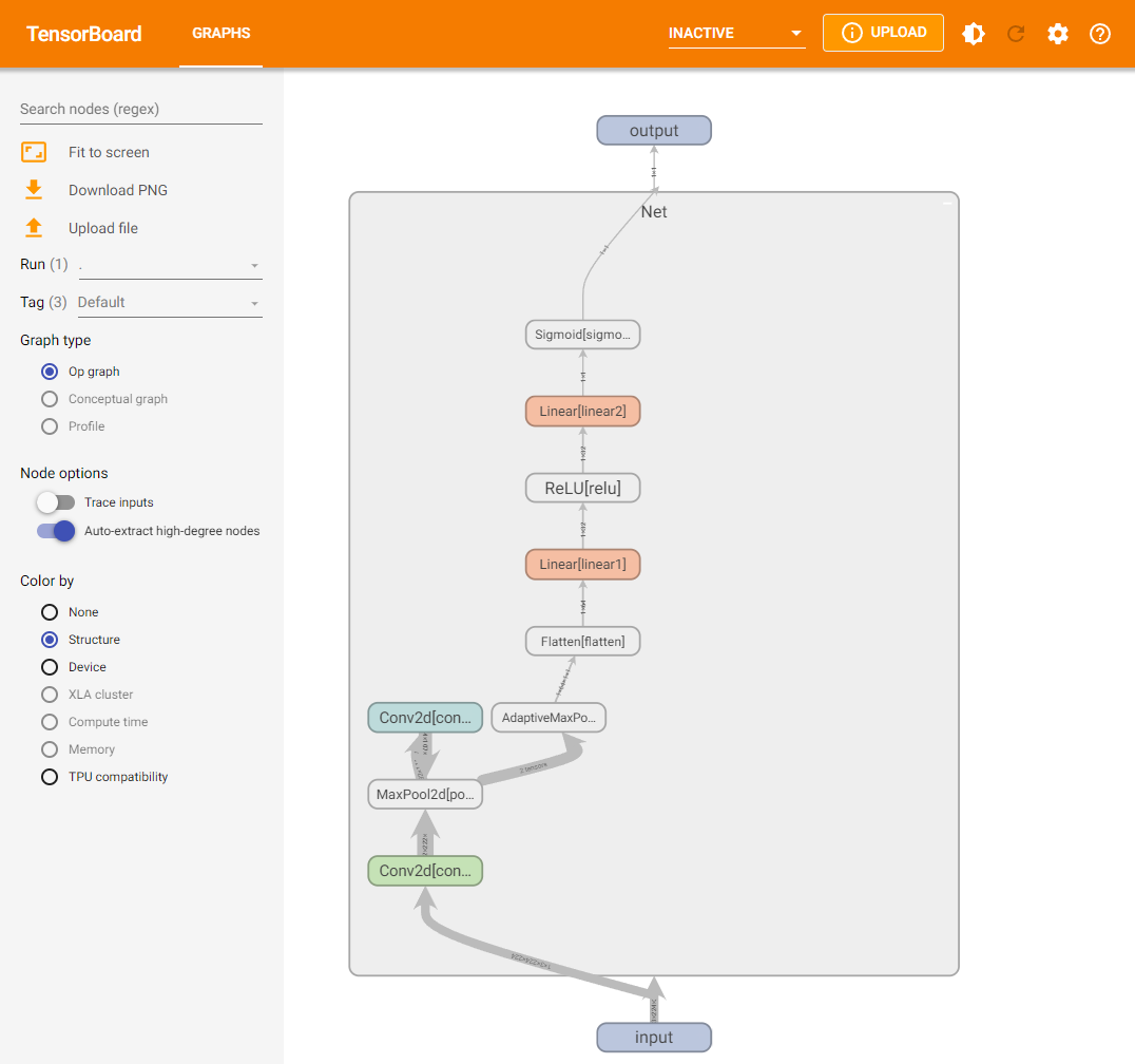
模型结构可视化:使用
add_graph方法,在TensorBoard下展示模型结构
import torch.nn as nnclass Net(nn.Module): def __init__(self): super(Net, self).__init__() self.conv1 = nn.Conv2d(in_channels=3,out_channels=32,kernel_size = 3) self.pool = nn.MaxPool2d(kernel_size = 2,stride = 2) self.conv2 = nn.Conv2d(in_channels=32,out_channels=64,kernel_size = 5) self.adaptive_pool = nn.AdaptiveMaxPool2d((1,1)) self.flatten = nn.Flatten() self.linear1 = nn.Linear(64,32) self.relu = nn.ReLU() self.linear2 = nn.Linear(32,1) self.sigmoid = nn.Sigmoid() def forward(self,x): x = self.conv1(x) x = self.pool(x) x = self.conv2(x) x = self.pool(x) x = self.adaptive_pool(x) x = self.flatten(x) x = self.linear1(x) x = self.relu(x) x = self.linear2(x) y = self.sigmoid(x) return ymodel = Net()print(model)Net( (conv1): Conv2d(3, 32, kernel_size=(3, 3), stride=(1, 1)) (pool): MaxPool2d(kernel_size=2, stride=2, padding=0, dilation=1, ceil_mode=False) (conv2): Conv2d(32, 64, kernel_size=(5, 5), stride=(1, 1)) (adaptive_pool): AdaptiveMaxPool2d(output_size=(1, 1)) (flatten): Flatten(start_dim=1, end_dim=-1) (linear1): Linear(in_features=64, out_features=32, bias=True) (relu): ReLU() (linear2): Linear(in_features=32, out_features=1, bias=True) (sigmoid): Sigmoid())
from torch.utils.tensorboard import SummaryWriterwriter = SummaryWriter('./runs')writer.add_graph(model, input_to_model = torch.rand(1, 3, 224, 224))writer.close()在当前目录下,执行tensorboard --logdir=./runs命令,打开TensorBoard可视化页面,看到模型网络结构。
-
图像可视化:
- 对于单张图片的显示使用
add_image - 对于多张图片的显示使用
add_images - 有时需要使用
torchvision.utils.make_grid将多张图片拼成一张图片后,用writer.add_image显示
- 对于单张图片的显示使用
-
连续变量可视化:使用
add_scalar方法,对连续变量(或时序变量)的变化过程进行可视化展示
for i in range(500): x = i y = x 2 writer.add_scalar("x", x, i) #日志中记录x在第step i 的值 writer.add_scalar("y", y, i) #日志中记录y在第step i 的值writer.close()Copy to clipboardErrorCopied- 参数分布可视化:使用
add_histogram方法,对参数(或变量)的分布进行可视化展示
import numpy as np# 创建正态分布的张量模拟参数矩阵def norm(mean, std): t = std * torch.randn((100, 20)) + mean return tfor step, mean in enumerate(range(-10, 10, 1)): w = norm(mean, 1) writer.add_histogram("w", w, step) writer.flush()writer.close()Copy to clipboardErrorCopied4 总结
本次任务,主要介绍了PyTorch可视化,包括可视化网络结构、CNN卷积层可视化和使用TensorBoard可视化训练过程。
- 使用
torchinfo库,可视化模型网络结构,展示模块信息(每一层的类型、输出shape和参数量)、模型整体的参数量、模型大小、一次前向或者反向传播需要的内存大小等。 - 使用
grad-cam库,可视化重要像素点,能够快速确定重要区域,进行可解释性分析或模型优化改进。 - 通过
TensorBoard工具,调用相关方法创建训练记录,可视化模型结构、图像、连续变量和参数分布等。