Android SensorManager部分源码解读

文档中心
Android SensorManger类部分源码解读

1.getRotationMatrix

1.1源码

/**     *      * Computes the inclination matrix I as well as the rotation matrix     * R transforming a vector from the device coordinate system to the     * world's coordinate system which is defined as a direct orthonormal basis,     * where:     * 
     *     *      * X is defined as the vector product Y.Z (It is tangential to     * the ground at the device's current location and roughly points East).
     * Y is tangential to the ground at the device's current location and     * points towards the magnetic North Pole.
     * Z points towards the sky and is perpendicular to the ground.
     * 
     *     *      *      * 
     *     *      * 
     *      * By definition:     * 
     * [0 0 g] = R * gravity (g = magnitude of gravity)     * 
     * [0 m 0] = I * R * geomagnetic (m = magnitude of     * geomagnetic field)     * 
     * R is the identity matrix when the device is aligned with the     * world's coordinate system, that is, when the device's X axis points     * toward East, the Y axis points to the North Pole and the device is facing     * the sky.     *     * 
     * I is a rotation matrix transforming the geomagnetic vector into     * the same coordinate space as gravity (the world's coordinate space).     * I is a simple rotation around the X axis. The inclination angle in     * radians can be computed with {@link #getInclination}.     * 
     *     *      * Each matrix is returned either as a 3x3 or 4x4 row-major matrix depending     * on the length of the passed array:     * 
     * If the array length is 16:     *     * 
     *   /  M[ 0]   M[ 1]   M[ 2]   M[ 3]  \     *   |  M[ 4]   M[ 5]   M[ 6]   M[ 7]  |     *   |  M[ 8]   M[ 9]   M[10]   M[11]  |     *   \  M[12]   M[13]   M[14]   M[15]  /     *
     *     * This matrix is ready to be used by OpenGL ES's     * {@link javax.microedition.khronos.opengles.GL10#glLoadMatrixf(float[], int)     * glLoadMatrixf(float[], int)}.     * 
     * Note that because OpenGL matrices are column-major matrices you must     * transpose the matrix before using it. However, since the matrix is a     * rotation matrix, its transpose is also its inverse, conveniently, it is     * often the inverse of the rotation that is needed for rendering; it can     * therefore be used with OpenGL ES directly.     * 
     * Also note that the returned matrices always have this form:     *     * 
     *   /  M[ 0]   M[ 1]   M[ 2]   0  \     *   |  M[ 4]   M[ 5]   M[ 6]   0  |     *   |  M[ 8]   M[ 9]   M[10]   0  |     *   \      000   1  /     *
     *     * 
     * If the array length is 9:     *     * 
     *   /  M[ 0]   M[ 1]   M[ 2]  \     *   |  M[ 3]   M[ 4]   M[ 5]  |     *   \  M[ 6]   M[ 7]   M[ 8]  /     *
     *     * 
     * 
     * The inverse of each matrix can be computed easily by taking its     * transpose.     *     * 
     * The matrices returned by this function are meaningful only when the     * device is not free-falling and it is not close to the magnetic north. If     * the device is accelerating, or placed into a strong magnetic field, the     * returned matrices may be inaccurate.     *     * @param R     * is an array of 9 floats holding the rotation matrix R when     * this function returns. R can be null.     * 
     *     * @param I     * is an array of 9 floats holding the rotation matrix I when     * this function returns. I can be null.     * 
     *     * @param gravity     * is an array of 3 floats containing the gravity vector expressed in     * the device's coordinate. You can simply use the     * {@link android.hardware.SensorEvent#values values} returned by a     * {@link android.hardware.SensorEvent SensorEvent} of a     * {@link android.hardware.Sensor Sensor} of type     * {@link android.hardware.Sensor#TYPE_ACCELEROMETER     * TYPE_ACCELEROMETER}.     * 
     *     * @param geomagnetic     * is an array of 3 floats containing the geomagnetic vector     * expressed in the device's coordinate. You can simply use the     * {@link android.hardware.SensorEvent#values values} returned by a     * {@link android.hardware.SensorEvent SensorEvent} of a     * {@link android.hardware.Sensor Sensor} of type     * {@link android.hardware.Sensor#TYPE_MAGNETIC_FIELD     * TYPE_MAGNETIC_FIELD}.     *     * @return true on success, false on failure (for     *  instance, if the device is in free fall). Free fall is defined as     *  condition when the magnitude of the gravity is less than 1/10 of     *  the nominal value. On failure the output matrices are not modified.     *     * @see #getInclination(float[])     * @see #getOrientation(float[], float[])     * @see #remapCoordinateSystem(float[], int, int, float[])     */    public static boolean getRotationMatrix(float[] R, float[] I,     float[] gravity, float[] geomagnetic) { // TODO: move this to native code for efficiency float Ax = gravity[0]; float Ay = gravity[1]; float Az = gravity[2]; // normsqA是向量点乘。 final float normsqA = (Ax * Ax + Ay * Ay + Az * Az); final float g = 9.81f; final float freeFallGravitySquared = 0.01f * g * g; if (normsqA < freeFallGravitySquared) {     // gravity less than 10% of normal value     return false; } final float Ex = geomagnetic[0]; final float Ey = geomagnetic[1]; final float Ez = geomagnetic[2]; float Hx = Ey * Az - Ez * Ay; float Hy = Ez * Ax - Ex * Az; float Hz = Ex * Ay - Ey * Ax; final float normH = (float) Math.sqrt(Hx * Hx + Hy * Hy + Hz * Hz); if (normH < 0.1f) {     // device is close to free fall (or in space?), or close to     // magnetic north pole. Typical values are  > 100.     return false; } final float invH = 1.0f / normH; Hx *= invH; Hy *= invH; Hz *= invH; final float invA = 1.0f / (float) Math.sqrt(Ax * Ax + Ay * Ay + Az * Az); Ax *= invA; Ay *= invA; Az *= invA; final float Mx = Ay * Hz - Az * Hy; final float My = Az * Hx - Ax * Hz; final float Mz = Ax * Hy - Ay * Hx; if (R != null) {     if (R.length == 9) {  R[0] = Hx;     R[1] = Hy;     R[2] = Hz;  R[3] = Mx;     R[4] = My;     R[5] = Mz;  R[6] = Ax;     R[7] = Ay;     R[8] = Az;     } else if (R.length == 16) {  R[0]  = Hx;    R[1]  = Hy;    R[2]  = Hz;   R[3]  = 0;  R[4]  = Mx;    R[5]  = My;    R[6]  = Mz;   R[7]  = 0;  R[8]  = Ax;    R[9]  = Ay;    R[10] = Az;   R[11] = 0;  R[12] = 0;     R[13] = 0;     R[14] = 0;    R[15] = 1;     } } if (I != null) {     // compute the inclination matrix by projecting the geomagnetic     // vector onto the Z (gravity) and X (horizontal component     // of geomagnetic vector) axes.     final float invE = 1.0f / (float) Math.sqrt(Ex * Ex + Ey * Ey + Ez * Ez);     final float c = (Ex * Mx + Ey * My + Ez * Mz) * invE;     final float s = (Ex * Ax + Ey * Ay + Ez * Az) * invE;     if (I.length == 9) {  I[0] = 1;     I[1] = 0;     I[2] = 0;  I[3] = 0;     I[4] = c;     I[5] = s;  I[6] = 0;     I[7] = -s;     I[8] = c;     } else if (I.length == 16) {  I[0] = 1;     I[1] = 0;     I[2] = 0;  I[4] = 0;     I[5] = c;     I[6] = s;  I[8] = 0;     I[9] = -s;     I[10] = c;  I[3] = I[7] = I[11] = I[12] = I[13] = I[14] = 0;  I[15] = 1;     } } return true;    } 
1.2原理
1.2.1传感器坐标系
 通常，传感器框架使用标准的 3 轴坐标系来表示数据值。对于大多数传感器，当设备处于自然屏幕方向时，会相对于设备屏幕来定义坐标系（参见图 1）。当设备处于自然屏幕方向时，X 轴为水平向右延伸，Y 轴为垂直向上延伸，Z 轴为垂直于屏幕向外延伸。在此坐标系中，屏幕后面的坐标将具有负 Z 值。以下传感器使用此坐标系：加速度传感器、重力传感器、陀螺仪、线性加速度传感器、地磁场传感器。
   
图1 Sensor API 使用的坐标系（相对于设备）
注1：在图形学中，这种坐标系叫做物体坐标系。物体坐标与物体绑定，不会因为物体在世界坐标系中状态的改变而改变。世界坐标系可以简单理解为可以描述其他所有坐标系或者物体的位置的最大坐标系。而安卓中的世界坐标系，经过验证，可以确定为：X轴正向为正北，Y轴正向为正东，Z轴正向指向天空（与重力方向相反）。
注2：设备的自然屏幕方向不一定总是竖屏。通常情况下平板设备一般为横屏，而传感器坐标系始终基于自然屏幕方向。
注3：图1来自谷歌开发文档，侵删。
1.2.2坐标基本变换（二维）
1.2.2.1二维平移
 将平移距离Tx和Ty加到原始坐标(x,y)上获得一个新的坐标位置(x’,y’)，可以实现一个二维位置的平移，写成矩阵形式为：
  $\begin{bmatrix} x' \\\\ y' \end{bmatrix}= \begin{bmatrix} x \\\\ y \end{bmatrix}+ \begin{bmatrix} t_x \\\\ t_y \end{bmatrix}$ 
1.2.2.2二维旋转
 在极坐标系中，r是点到原点的固定距离，角度φ是点(x,y)的原始角度位置与水平线的夹角，θ是旋转角（逆时针为正），则旋转后的坐标(x’,y’)可以表示为：
  $\begin{cases} x'=r(cos \theta + \phi ) =rcos \phi cos \theta -rsin \phi sin \theta \\\\ y'=r(sin \theta + \phi ) =rcos \phi sin \theta +rsin \phi cos \theta \end{cases}$ 
  在极坐标系中，点的原始坐标为：
  $\theta ,y=rsin \theta$ 
  代入得：
  $\begin{cases} x'=xcos \theta -ysin \theta \\\\ y'=xsin \theta +ycos \theta \end{cases}$ 
  旋转矩阵R为：
  $\theta )= \begin{bmatrix} cos \theta &-sin \theta \\\\ sin \theta & cos \theta \end{bmatrix}$ 
 写出矩阵形式为：
  $\begin{bmatrix} x' \\\\ y' \end{bmatrix}= R \cdot \begin{bmatrix} x \\\\ y \end{bmatrix}$ 
1.2.2.3二维缩放
 改变一个对象的大小，可以使用缩放变化。一个简单的二维缩放操作可以通过将缩放系数Sx和Sy与对象坐标位置(x,y)相乘而得，写成矩阵形式为：
  $\begin{bmatrix} x' \\\\ y' \end{bmatrix}= \begin{bmatrix} s_x&0 \\\\ 0&s_y \end{bmatrix} \begin{bmatrix} x \\\\ y \end{bmatrix}$ 
 当Sx和Sy相同时，就会产生保持对象相对比例的一致缩放，不同时就叫差值缩放。
1.2.3齐次坐标
 许多图形应用涉及到几何变化的顺序，在1.2.2节中我们已经看到，每个基本变换（平移、旋转和缩放）都可以表示为普通矩阵形式：
  $P'=M_1 \cdot P+M_2$ 
 坐标位置P’和P表示为列向量，矩阵M1是一个包含乘法系数的2×2矩阵，M2是包含平移项的两元素列矩阵。对于平移，M1是单位矩阵。对于旋转或缩放，M2包含与基准点或缩放固定点相关的平移项。为了利用这个公式产生先缩放、再旋转、后平移这样的变化顺序，必须一步一步地计算变换的坐标。而实际上，更有效的做法应该是将变换组合，从而直接从初始坐标得到最后的坐标位置，这样就消除了中间坐标值的计算。因此，需要重组等式以消除M2中与平移项相关的矩阵加法。
 如果将2×2矩阵表达式扩充为3×3矩阵，就可以把二维几何变化的乘法和平移项组合成单一矩阵表示。这时将变换矩阵的第三列用于平移项，而所有的变换公式可表达为矩阵乘法。但为了这样操作，必须解释二维坐标位置到三元列向量的矩阵表示。标准的实现技术是将二维坐标(X,Y)扩充到三维表示(Xh,Yh,h)，称为齐次坐标。这里的齐次参数h是一个非零值，因此
  $\frac {x_h} {h} ,y = \frac {y_h} {h}$ 
  这样，普通的二维齐次坐标表示可写为(h·x,h·y,h)。对于二维几何变换，可以把齐次参数h取为任何非零值。因而，对于每个坐标点(x,y)，可以有无数个等价的齐次表达式。最方便的选择是简单地设置为h=1。因此每个二维位置都可以用齐次坐标(x,y,1)来表示。h的其他值也是需要的，例如在三维观察变换的矩阵公式中。
 源码中之所以出现4×4的三维旋转矩阵，用的就是齐次坐标这一概念。
1.2.4坐标系间的变换（三维旋转）
 我们可以围绕空间的任意轴旋转一个对象，但绕平行于坐标轴的轴的旋转是最容易处理的。我们同样可以利用围绕坐标轴旋转（结合适当的平移）的复合结果来表示任意一种旋转。因此，我们先考虑坐标轴的旋转操作，然后讨论其他旋转轴所需的计算。
 旋转分为两种，一种是旋转物体，一种是旋转坐标系，前者称为主动旋转，后者称为被动旋转。因为在Android中旋转主要是旋转手机，即旋转物体坐标系，所以以下只研究被动旋转。
 为了方便理解，我们首先从二维旋转矩阵开始。如图2，同样的一个点，虽然位置不变，但是在旋转前和旋转后的坐标系中，坐标是不一样的。设旋转前为(x,y)，旋转后为(x’,y’)。
   
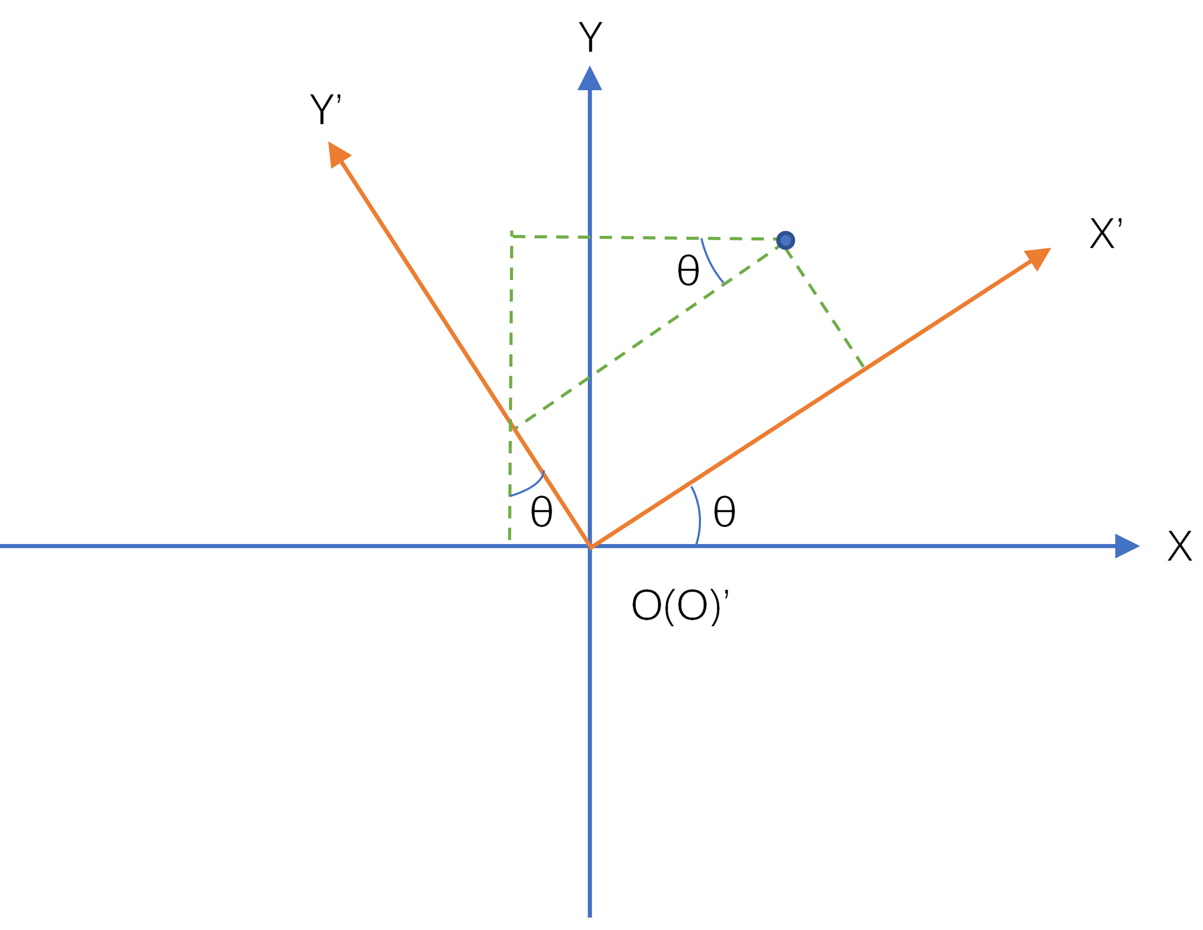
图2 二维旋转坐标系示意图 
 由1.2.2.2中公式可以得到，旋转矩阵R为：
  $\theta )= \begin{bmatrix} cos \theta &sin \theta \\\\ -sin \theta &cos \theta \end{bmatrix}$ 
  因为逆时针旋转坐标系相当于顺时针旋转点，所以θ相反。至此，我们可以将2D平面的旋转问题提升到3D空间的旋转问题，即分别绕三个轴作类似2D的旋转变换。需要额外注意的两个的问题是：
①通常，如果沿着坐标轴的正半轴观察原点，那么绕坐标轴的逆时针旋转为正向旋转；
②空间坐标系的旋转关系(复合结果)与各坐标轴的旋转顺序相关。
 绕Z轴的二维坐标系旋转很容易推广到三维：
  $\begin{cases} x'=xcos \theta +ysin \theta \\\\ y'=-xsin \theta +ycos \theta \\\\ z'=z \end{cases}$ 
 同理，绕X轴和绕Y轴的对应坐标关系如下，可由上式用X->Y->Z->X顺序循环替换（将X替换为Y，将Y替换为Z，将Z替换为X）得到：
  $\begin{cases} y'=ycos \theta +zsin \theta \\\\ z'=-ysin \theta +zcos \theta \\\\ x'=x \end{cases}$ 
 $\begin{cases} z'=zcos \theta +xsin \theta \\\\ x'=-zsin \theta +xcos \theta \\\\ y'=y \end{cases}$ 
 我们假设坐标系O-XYZ依次绕自身Z轴、X轴、Y轴（Z-X-Y构成了一个旋转序列）分别逆时针转θ1，θ2，θ3后可以与坐标系O’-X’Y’Z’重合，则空间中某点M在这两个坐标系中的描述关系如下：
  $\begin{bmatrix} x' \\\\ y' \\\\ z' \end{bmatrix}= \begin{bmatrix} cos \theta_3&0&-sin \theta_3 \\\\ 0&1&0 \\\\ sin \theta_3&0& cos \theta_3 \end{bmatrix} \begin{bmatrix} 1&0&0 \\\\ 0& cos \theta_2&sin \theta_2 \\\\ 0&-sin \theta_2&cos \theta_2 \end{bmatrix} \begin{bmatrix} cos \theta_1&sin \theta_1&0 \\\\ -sin \theta_1&cos \theta_1&0 \\\\ 0&0&1 \end{bmatrix} \begin{bmatrix} x \\\\ y \\\\ z \end{bmatrix}$ 
1.3代码解释
 三维空间中只需要3个基向量即可表示空间中所有的向量，想要获得的3*3旋转矩阵R实际上是一组规范正交基。也就是说，我们希望通过地磁和重力获得这样一个R矩阵，当设备满足以下条件：
 ①设备屏幕所在的平面和地面所在的平面平行；
 ②设备的自然屏幕方向（Y轴正向）与地磁方向（正北）相同；
 ③设备屏幕朝向天空（此时Z轴正向与重力方向相反）；
此时的设备（物体坐标系）与世界坐标系对齐，R为单位矩阵。
 I矩阵也是一个旋转矩阵，它的作用是将地磁向量转换到与重力（世界坐标空间）相同的坐标空间。I只是一个绕X轴的旋转矩阵，它也可以使用下面这个函数获得。
getInclination(float[])
 虽然利用重力和地磁可以唯一确定一个世界坐标系，但是重力方向和地磁方向却不一定是垂直的。为了获得一组规范正交基（世界坐标系），还需要再进行一次叉乘计算。具体过程如下：
 ①通过向量E（地磁向量）和向量A（与重力向量大小相等，方向相反）的叉乘（E×A）确定东西方向的向量H。向量H指向正东，且由叉乘的性质可知，该向量一定与重力向量A和地磁向量E垂直。
 ②将向量H和向量A规范化。
 ③向量A与向量H的叉乘（A×H）可以得到南北方向的向量M。向量M指向正北，且一定与向量A和向量H垂直，此时便得到了由向量H、向量M和向量A组成的一组规范正交基。
 ④矩阵R就是由向量H、向量M和向量A组成的。
  $^\mathsf{T}$ 
  矩阵I的计算步骤也是非常好理解的，它的目的就是获得从物体坐标系到世界坐标系的一个简单旋转矩阵。设坐标系原点为O，由于地磁向量在MOA（YOZ）平面，所以该旋转矩阵就是绕H（X）轴的一个旋转矩阵。具体公式在1.2.2中介绍过了，就不再赘述了。
2.getOrientation
2.1源码
 /**     * Computes the device's orientation based on the rotation matrix.     *      * When it returns, the array values are as follows:     * 
     * values[0]: Azimuth, angle of rotation about the -z axis.     *  This value represents the angle between the device's y     *  axis and the magnetic north pole. When facing north, this     *  angle is 0, when facing south, this angle is π.     *  Likewise, when facing east, this angle is π/2, and     *  when facing west, this angle is -π/2. The range of     *  values is -π to π.
     * values[1]: Pitch, angle of rotation about the x axis.     *  This value represents the angle between a plane parallel     *  to the device's screen and a plane parallel to the ground.     *  Assuming that the bottom edge of the device faces the     *  user and that the screen is face-up, tilting the top edge     *  of the device toward the ground creates a positive pitch     *  angle. The range of values is -π to π.
     * values[2]: Roll, angle of rotation about the y axis. This     *  value represents the angle between a plane perpendicular     *  to the device's screen and a plane perpendicular to the     *  ground. Assuming that the bottom edge of the device faces     *  the user and that the screen is face-up, tilting the left     *  edge of the device toward the ground creates a positive     *  roll angle. The range of values is -π/2 to π/2.
     * 
     *      * Applying these three rotations in the azimuth, pitch, roll order     * transforms an identity matrix to the rotation matrix passed into this     * method. Also, note that all three orientation angles are expressed in     * radians.     *     * @param R     * rotation matrix see {@link #getRotationMatrix}.     *     * @param values     * an array of 3 floats to hold the result.     *     * @return The array values passed as argument.     *     * @see #getRotationMatrix(float[], float[], float[], float[])     * @see GeomagneticField     */    public static float[] getOrientation(float[] R, float[] values) { /*  * 4x4 (length=16) case:  *   /  R[ 0]   R[ 1]   R[ 2]   0  \  *   |  R[ 4]   R[ 5]   R[ 6]   0  |  *   |  R[ 8]   R[ 9]   R[10]   0  |  *   \      000   1  /  *  * 3x3 (length=9) case:  *   /  R[ 0]   R[ 1]   R[ 2]  \  *   |  R[ 3]   R[ 4]   R[ 5]  |  *   \  R[ 6]   R[ 7]   R[ 8]  /  *  */ if (R.length == 9) {     values[0] = (float) Math.atan2(R[1], R[4]);     values[1] = (float) Math.asin(-R[7]);     values[2] = (float) Math.atan2(-R[6], R[8]); } else {     values[0] = (float) Math.atan2(R[1], R[5]);     values[1] = (float) Math.asin(-R[9]);     values[2] = (float) Math.atan2(-R[8], R[10]); } return values;    }
2.2原理
2.2.1 Android 设备方向


方位角（绕 Z轴旋转的角度）。此为设备当前指南针方向与磁北向之间的角度。如果设备的上边缘面朝磁北向，则方位角为 0 度；如果上边缘朝南，则方位角为 180 度。与之类似，如果上边缘朝东，则方位角为 90 度；如果上边缘朝西，则方位角为 270 度。


俯仰角（绕 X轴旋转的角度）。此为平行于设备屏幕的平面与平行于地面的平面之间的角度。如果将设备与地面平行放置，且其下边缘最靠近您，同时将设备上边缘向地面倾斜，则俯仰角将变为正值。沿相反方向倾斜（将设备上边缘向远离地面的方向移动）将使俯仰角变为负值。值的范围为 -180 度到 180 度。


倾侧角（绕 Y 轴旋转的角度）。此为垂直于设备屏幕的平面与垂直于地面的平面之间的角度。如果将设备与地面平行放置，且其下边缘最靠近您，同时将设备左边缘向地面倾斜，则侧倾角将变为正值。沿相反方向倾斜（将设备右边缘移向地面）将使侧倾角变为负值。值的范围为 -90 度到 90 度。


2.2.2 欧拉角
 欧拉角的核心思想是：一个坐标系可以用另一个参考坐标系的三次空间旋转来表达。旋转坐标系的方法有两种：
 ① Proper Euler angles：第一次与第三次旋转相同的坐标轴。
 ② Tait-Bryan angles：依次旋转三个不同的坐标轴。
 对于每个旋转序列（不同旋转序列会产生不同的旋转矩阵），又分为内在旋转和外在旋转两种方式。设有两个坐标系O-XYZ和O-X’Y’Z’，其中O-XYZ是固定不动的参考系，O-X’Y’Z’是需要被旋转的坐标系，初始时两个坐标系重合。内在旋转指每次旋转的旋转轴都是上次变换后新系O-X’Y’Z’的坐标轴，外在旋转是指每次旋转的旋转轴都是固定参考系O-XYZ的坐标轴。外在旋转等效于内在旋转的旋转序列的倒序。
2.2.3 Android使用的被动旋转矩阵
 下面给出Android源码中使用的被动旋转矩阵：
  $R_{Z_1X_2Y_3}= \begin{bmatrix} cos \phi cos \psi -sin \phi sin \psi sin \theta &sin \phi cos \theta &cos \phi sin \psi +sin \phi cos \psi sin \theta \\\\ -sin \phi cos \psi -cos \phi sin \psi sin \theta & cos \phi cos \theta &-sin \phi sin \psi +cos \phi cos \psi sin \theta \\\\ -sin \psi cos \theta &-sin \theta & cos \psi cos \theta \end{bmatrix}$ 
  上式中，φ为方位角，θ为俯仰角，ψ为倾侧角。
 如果问，为什么是旋转序列为ZXY，理由并不复杂：ZXY对应AHM，在getRotationMatrix函数中，向量H是根据向量A计算出的，向量M又是根据向量H和向量A计算出的。所以对于旋转来说，先确定Z轴，再确定X轴，最后确定Y轴就不言而喻了。
2.3代码解释
 getOrientation函数的代码比较简单，没有什么复杂的逻辑，只需要将代码与2.2.3中给出的公式对比一下即可。这里只解释一下Math.atan2函数的使用，atan2的具体公式如图。
   
图3 atan2公式
3.getRotationMatrixFromVector
3.1源码
/** Helper function to convert a rotation vector to a rotation matrix.     *  Given a rotation vector (presumably from a ROTATION_VECTOR sensor), returns a     *  9  or 16 element rotation matrix in the array R.  R must have length 9 or 16.     *  If R.length == 9, the following matrix is returned:     *      *   /  R[ 0]   R[ 1]   R[ 2]   \     *   |  R[ 3]   R[ 4]   R[ 5]   |     *   \  R[ 6]   R[ 7]   R[ 8]   /     *
     * If R.length == 16, the following matrix is returned:     * 
     *   /  R[ 0]   R[ 1]   R[ 2]   0  \     *   |  R[ 4]   R[ 5]   R[ 6]   0  |     *   |  R[ 8]   R[ 9]   R[10]   0  |     *   \  0001  /     *
     *  @param rotationVector the rotation vector to convert     *  @param R an array of floats in which to store the rotation matrix     */    public static void getRotationMatrixFromVector(float[] R, float[] rotationVector) { float q0; float q1 = rotationVector[0]; float q2 = rotationVector[1]; float q3 = rotationVector[2]; if (rotationVector.length >= 4) {     q0 = rotationVector[3]; } else {     q0 = 1 - q1 * q1 - q2 * q2 - q3 * q3;     q0 = (q0 > 0) ? (float) Math.sqrt(q0) : 0; } float sq_q1 = 2 * q1 * q1; float sq_q2 = 2 * q2 * q2; float sq_q3 = 2 * q3 * q3; float q1_q2 = 2 * q1 * q2; float q3_q0 = 2 * q3 * q0; float q1_q3 = 2 * q1 * q3; float q2_q0 = 2 * q2 * q0; float q2_q3 = 2 * q2 * q3; float q1_q0 = 2 * q1 * q0; if (R.length == 9) {     R[0] = 1 - sq_q2 - sq_q3;     R[1] = q1_q2 - q3_q0;     R[2] = q1_q3 + q2_q0;     R[3] = q1_q2 + q3_q0;     R[4] = 1 - sq_q1 - sq_q3;     R[5] = q2_q3 - q1_q0;     R[6] = q1_q3 - q2_q0;     R[7] = q2_q3 + q1_q0;     R[8] = 1 - sq_q1 - sq_q2; } else if (R.length == 16) {     R[0] = 1 - sq_q2 - sq_q3;     R[1] = q1_q2 - q3_q0;     R[2] = q1_q3 + q2_q0;     R[3] = 0.0f;     R[4] = q1_q2 + q3_q0;     R[5] = 1 - sq_q1 - sq_q3;     R[6] = q2_q3 - q1_q0;     R[7] = 0.0f;     R[8] = q1_q3 - q2_q0;     R[9] = q2_q3 + q1_q0;     R[10] = 1 - sq_q1 - sq_q2;     R[11] = 0.0f;     R[12] = R[13] = R[14] = 0.0f;     R[15] = 1.0f; }    } 
3.2原理
3.2.1四元数
3.2.1.1定义
 四元数与复数的定义非常类似，唯一的区别就是四元数一共有三个虚部，而复数只有一个，所有的四元数q∈H（H代表四元数的发现者William Rowan）都可以写成下面这种形式：
  $\vec{i}+c \vec{j}+d \vec{k},(a,b,c,d∈ \mathbb{R})$ 
 以下q均指四元数,且特指上式。其中
  $\vec{i^2}= \vec{j^2}=\vec{k^2}=\vec{i}\vec{j}\vec{k}=-1$ 
  与复数类似，因为四元数就是对于基{1,i,j,k}的线性组合，四元数也可以写成向量的形式：
  $\begin{bmatrix} a \\\\ b \\\\ c \\\\ d \end{bmatrix}$ 
  除此之外，我们经常将四元数的实部与虚部分开，并用一个三维的向量来表示虚部，将它表示为标量和向量的有序对形式：
  $\begin{bmatrix} s,\boldsymbol{v} \end{bmatrix}.(\boldsymbol{v}= \begin{bmatrix} x \\\\ y \\\\ z \end{bmatrix},s,x,y,z \in \mathbb{R} )$ 
 如果s=0，则我们称q为一个纯四元数。
 共轭四元数：我们定义q的共轭为（q* 读作 q star）
  $q^*=a-b \vec{i}-c \vec{j}-d \vec{k}$ 
3.2.1.2性质
模长
 $\sqrt{a^2+b^2+c^2+d^2} 或||q||= \sqrt{s^2+ \boldsymbol{v} \cdot \boldsymbol{v}} (\boldsymbol{v} \cdot \boldsymbol{v}= || \boldsymbol{v}||^2)$ 
加减法
 与复数一样，实部与实部相加减，对应的虚部与虚部相加减。
标量与四元数相乘
 符合交换律，q乘以一个标量s，所有的部分都要乘以s。
四元数乘法
 不符合交换律，有左乘和右乘的区别，满足结合律和分配律。设两个四元数分别为：
  $q_1=a_1+b_1 \vec{i}+c_1 \vec{j}+d_1 \vec{k},(a_1,b_1,c_1,d_1∈ \mathbb{R}) \\\\ q_2=a_2+b_2 \vec{i}+c_2 \vec{j}+d_2 \vec{k},(a_2,b_2,c_2,d_2∈ \mathbb{R})$ 
  那么它们的乘积为：
  $\begin{aligned} q_1q_2=&(a_1+b_1 \vec{i}+c_1 \vec{j}+d_1 \vec{k})(a_2+b_2 \vec{i}+c_2 \vec{j}+d_2 \vec{k}) \\\\ =&a_1a_2+a_1b_2 \vec{i}+a_1c_2 \vec{j}+a_1d_2 \vec{k}+ \\\\ &b_1a_2 \vec{i}+b_1b_2 \vec{i}^2+b_1c_2 \vec{i}\vec{j}+a_1d_2 \vec{i}\vec{k}+ \\\\ &c_1a_2 \vec{j}+c_1b_2 \vec{j}\vec{i}+c_1c_2 \vec{j}^2+c_1d_2 \vec{j}\vec{k}+ \\\\ &d_1a_2 \vec{k}+d_1b_2 \vec{k}\vec{i}+d_1c_2 \vec{k}\vec{j}+d_1d_2 \vec{k}^2 \end{aligned}$ 
 这样的乘法看起来十分的凌乱，但是我们可以根据
  $\vec{i^2}= \vec{j^2}=\vec{k^2}=\vec{i}\vec{j}\vec{k}=-1$ 
  化简这个定义，可以得到这样一个表格



X
1
i
j
k




1
1
i
j
k


i
i
-1
k
-j


j
j
-k
-1
i


k
k
j
-i
-1



 表格最左列中一个元素右乘以顶行中一个元素的结果就位于这连个元素行列的交叉处。利用这个表格，我们就能进一步化简四元数乘积的结果：
  $\begin{aligned} q_1q_2=&a_1a_2+a_1b_2 \vec{i}+a_1c_2 \vec{j}+a_1d_2 \vec{k}+ \\\\ & b_1a_2 \vec{i}-b_1b_2+b_1c_2 \vec{k}-a_1d_2 \vec{j}+ \\\\ & c_1a_2 \vec{j}-c_1b_2 \vec{k}-c_1c_2+c_1d_2 \vec{i}+ \\\\ & d_1a_2 \vec{k}+d_1b_2 \vec{j}-d_1c_2 \vec{i}-d_1d_2 \\\\ =&(a_1a_2-b_1b_2-c_1c_2-d_1d_2)+ \\\\ &(b_1a_2+a_1b_2-d_1c_2+c_1d_2) \vec{i}+ \\\\ &(c_1a_2+d_1b_2+a_1c_2-b_1d_2) \vec{j}+ \\\\ &(d_1a_2-c_1b_2+b_1c_2+a_1d_2) \vec{k} \\\\ = & \begin{bmatrix} a_1 & -b_1 & -c_1 & -d_1 \\\\ b_1 & a_1 & -d_1 & c_1 \\\\ c_1 & d_1 & a_1 & -b_1 \\\\ d_1 & -c_1 & b_1 & a_1 \end{bmatrix} \begin{bmatrix} a_2 \\\\ b_2 \\\\ c_2 \\\\ d_2 \end{bmatrix} \end{aligned}$ 
  这里直接给出：
  $q_2q_1= \begin{bmatrix} a_2 & -b_2 & -c_2 & -d_2 \\\\ b_2 & a_2 & d_2 & -c_2 \\\\ c_2 & -d_2 & a_2 & b_2 \\\\ d_2 & c_2 & -b_2 & a_2 \end{bmatrix} \begin{bmatrix} a_1 \\\\ b_1 \\\\ c_1 \\\\ d_1 \end{bmatrix}$ 
  如果令
  $\boldsymbol{v}=\begin{bmatrix} b_1 \\\\ c_1 \\\\ d_1 \end{bmatrix}, \boldsymbol{u}=\begin{bmatrix} b_2 \\\\ c_2 \\\\ d_2 \end{bmatrix}$ 
  那么
  $\begin{aligned} \boldsymbol{v} \cdot \boldsymbol{u}&=b_1b_2+c_1c_2+d_1d_2 \\\\ \boldsymbol{v} \times \boldsymbol{u}&=(c_1d_2-d_1c_2) \vec{i}-(b_1d_2-d_1b_2) \vec{j}+(b_1c_2-c_1b_2) \vec{k} \end{aligned}$ 
  则
  $q_1q_2=[a_1a_2- \boldsymbol{v} \cdot \boldsymbol{u},a_1 \boldsymbol{u}+a_2 \boldsymbol{v}+ \boldsymbol{v} \times \boldsymbol{u}]$ 
  这个结果也叫Graßmann 积 (Graßmann Product)。
逆运算
 我们规定 ：
  $qq^{-1}=q^{-1}q=1(q \neq 0)$ 
共轭四元数相乘
 使用Graßmann 积可得：
  $\begin{aligned} qq^* &=[s, \boldsymbol{v}] \cdot [s, - \boldsymbol{v}] \\\\ &=[s^2+ \boldsymbol{v} \cdot \boldsymbol{v},0] \end{aligned}$ 
  可以看到，这最终的结果是一个实数，而它正是四元数模长的平方
  $s^2+x^2+y^2+z^2=||q||^2$ 
  同时可得（证明略）：
  $q^*q=qq^*$ 
共轭四元数与四元数的逆
 证明略，公式如下：
  $q^{-1}= \frac {q^*} {||q||^2}$ 
  如果q的模为1，则q为单位四元数。
3.2.2 3D旋转公式
向量型
 证明略，这里直接给出罗德里格斯（Rodrigues）旋转公式的定义。3D空间中任意一个向量V沿着单位向量u旋转θ角度之后的向量V‘为：
  $\boldsymbol{v'}= \boldsymbol{v}cos \theta +(1- cos \theta)( \boldsymbol{u} \cdot \boldsymbol{v}) \boldsymbol{u}+( \boldsymbol{u} \times \boldsymbol{v})sin \theta$ 
四元数型
下面给出使用四元数后的旋转公式定义，证明略。任意向量v沿着以单位向量定义的旋转轴u旋转θ度之后的v’可以使用四元数乘法获得。令
  $\boldsymbol{v}=[0,v],q=[cos( \frac{1}{2} \theta), sin(\frac{1}{2} \theta) \boldsymbol{u}]$ 
  则：
  $\boldsymbol{v'}=qvq^*=qvq^{-1}$ 
 令
  $\frac{1}{2} \theta), b=sin( \frac{1}{2} \theta)u_x, c=sin( \frac{1}{2} \theta)u_y, d=sin( \frac{1}{2} \theta)u_z$ 
  那么，它的矩阵形式为：
  $\begin{bmatrix} 1-2c^2-2d^2 & 2bc-2ad & 2ac+2bd \\\\ 2bc+2ad & 1-2b^2-2d^2 & 2cd-2ab \\\\ 2bd-2ac & 2ab+2cd & 1-2b^2-2c^2 \end{bmatrix}v$ 
3.2.3旋转矢量传感器
 旋转矢量传感器获得的三个元素表示如下：
  $\cdot sin( \frac{1}{2} \theta) \\\\ y \cdot sin( \frac{1}{2} \theta) \\\\ z \cdot sin( \frac{1}{2} \theta)$ 
  旋转矢量的大小等于 sin(θ/2)，并且旋转矢量的方向等于旋转轴的方向。实际上，旋转矢量就是单位四元数（cos(θ/2)、xsin(θ/2)、ysin(θ/2)、z*sin(θ/2)）的最后三个分量。
 大部分情况下，旋转矢量传感器获得的数据都是根据陀螺仪计算出来的。
 这是一段Android开发者文档中利用陀螺仪计算旋转矢量的源码（Kotlin）：
// Create a constant to convert nanoseconds to seconds.private val NS2S = 1.0f / 1000000000.0fprivate val deltaRotationVector = FloatArray(4) { 0f }private var timestamp: Float = 0foverride fun onSensorChanged(event: SensorEvent?) {    // This timestep's delta rotation to be multiplied by the current rotation    // after computing it from the gyro sample data.    if (timestamp != 0f && event != null) { val dT = (event.timestamp - timestamp) * NS2S // Axis of the rotation sample, not normalized yet. var axisX: Float = event.values[0] var axisY: Float = event.values[1] var axisZ: Float = event.values[2] // Calculate the angular speed of the sample val omegaMagnitude: Float = sqrt(axisX * axisX + axisY * axisY + axisZ * axisZ) // Normalize the rotation vector if it's big enough to get the axis // (that is, EPSILON should represent your maximum allowable margin of error) if (omegaMagnitude > EPSILON) {     axisX /= omegaMagnitude     axisY /= omegaMagnitude     axisZ /= omegaMagnitude } // Integrate around this axis with the angular speed by the timestep // in order to get a delta rotation from this sample over the timestep // We will convert this axis-angle representation of the delta rotation // into a quaternion before turning it into the rotation matrix. val thetaOverTwo: Float = omegaMagnitude * dT / 2.0f val sinThetaOverTwo: Float = sin(thetaOverTwo) val cosThetaOverTwo: Float = cos(thetaOverTwo) deltaRotationVector[0] = sinThetaOverTwo * axisX deltaRotationVector[1] = sinThetaOverTwo * axisY deltaRotationVector[2] = sinThetaOverTwo * axisZ deltaRotationVector[3] = cosThetaOverTwo    }    timestamp = event?.timestamp?.toFloat() ?: 0f    val deltaRotationMatrix = FloatArray(9) { 0f }    SensorManager.getRotationMatrixFromVector(deltaRotationMatrix, deltaRotationVector);    // User code should concatenate the delta rotation we computed with the current rotation    // in order to get the updated rotation.    // rotationCurrent = rotationCurrent * deltaRotationMatrix;}
结合上面给出的四元数型3D旋转公式，这段代码并不难理解，给出这段代码的用途是方便读者理解getRotationMatrixFromVector中使用的旋转矢量是怎么来的。
3.3代码解释
 这个函数的源码也相当简单，难就难在理解返回值的意义。通过3.2中的大量原理公式，可以得出，返回值就是罗德里格斯公式的四元数矩阵形式的旋转矩阵。
参考文档
1.Andriod 源码：SensorManager.java - Android Code Search
2.Android 开发者文档 ：传感器 | Android 开发者 | Android Developers (google.cn)
3.计算机图形学 第5章 几何变换 ：计算机图形学第三版_百度百科 (baidu.com)
4.欧拉角：Euler angles - Wikipedia
5.四元数与三维旋转： Krasjet/quaternion (github.com)
联系方式
本文仅供参考学习使用。如果书写有误或者侵犯了相关作者的权益，请联系我。
QQ：572249217。
EMAIL：572249217@qq.com
Android SensorManager部分源码解读

Android SensorManger类部分源码解读

1.getRotationMatrix

1.1源码

1.2原理

1.2.1传感器坐标系

1.2.2坐标基本变换（二维）

1.2.2.1二维平移

1.2.2.2二维旋转

1.2.2.3二维缩放

1.2.3齐次坐标

1.2.4坐标系间的变换（三维旋转）

1.3代码解释

2.getOrientation

2.1源码

2.2原理

2.2.1 Android 设备方向

2.2.2 欧拉角

2.2.3 Android使用的被动旋转矩阵

2.3代码解释

3.getRotationMatrixFromVector

3.1源码

3.2原理

3.2.1四元数

3.2.1.1定义

3.2.1.2性质

模长

加减法

标量与四元数相乘

四元数乘法

逆运算

共轭四元数相乘

共轭四元数与四元数的逆

3.2.2 3D旋转公式

向量型

四元数型

3.2.3旋转矢量传感器

3.3代码解释

参考文档

联系方式

相关问题

公告

标签
