python 根据cartopy插件出气象等值线高度场图片

最近工作需要根据nc文件中要素出一张500hap高度场+850hpa风+850hpa相对湿度图片,

网上查找资料几天终于做出来了，下面直接上代码和效果图

import numpy as npimport matplotlib.pyplot as pltimport matplotlib as mplimport scipy.ndimage as ndimageimport xarray as xrimport cartopy.crs as ccrsimport cartopy.io.shapereader as shpreaderimport cartopy.feature as cfeaturefrom itertools import chainfrom cartopy.mpl.ticker import LongitudeFormatter, LatitudeFormatter# 打开文件path = 'D:/file/wrfprs_d01.2022040508.f15.nc'ds = xr.open_dataset(path)lat = ds['NLAT_GDS3_SFC']  # 维度lon = ds['ELON_GDS3_SFC']  # 经度hght = ds['HGT_GDS3_ISBL'].sel(lv_ISBL2=500)  # 高度# avor = ds['ABS_V_GDS3_ISBL'].sel(lv_ISBL2=500)#涡度avor = ds['TMP_GDS3_ISBL'].sel(lv_ISBL2=500)-273.15  # 温度# ds = xr.open_dataset(path)# 数据处理## 500hpa 数据# hgt_500 = ds['HGT_GDS3_ISBL']# temp_500 = ds['TMP_GDS3_ISBL']u_500 = ds['U_GRD_GDS3_ISBL']v_500 = ds['V_GRD_GDS3_ISBL']lons = ds['NLAT_GDS3_SFC'][0, :]lats = ds['ELON_GDS3_SFC'][:, 0]# hgt_500=hgt_500[0]*0.1 ## 单位换算为dagpm# temp_500 = temp_500[0]-273.15# u_500 = u_500[0]# v_500 = v_500[0]# hgt_500=hgt_500.sel(lv_ISBL2=500)*0.1 ## 单位换算为dagpm# temp_500 = temp_500.sel(lv_ISBL2=500)-273.15u_500 = u_500.sel(lv_ISBL2=500)v_500 = v_500.sel(lv_ISBL2=500)# 网格化 ，生成网格点坐标矩阵lons, lats = np.meshgrid(lons, lats)# 绘图# 一页4图# 设置投影方式，地图边界proj = ccrs.PlateCarree()  # 定义投影转换，后面都会用到，不必重复输入‘ccrs.PlateCarree()’# proj=ccrs.LambertConformal(central_longitude=120.0,central_latitude=45,standard_parallels=[40])# leftlon, rightlon, lowerlat, upperlat = (113,120,36,43)#113,120,36,43  70,140,15,55leftlon, rightlon, lowerlat, upperlat = (70,140,15,55)  # 113,120,36,43  70,140,15,55img_extent = [leftlon, rightlon, lowerlat, upperlat]# 建立画布fig = plt.figure(figsize=(12, 8))# 添加第一子图ax1 = fig.add_axes([0.1, 0.1, 0.8, 0.8], projection=proj)# contour_map(ax1,img_extent,10)# Smooth and re-plot the vorticity field 设置色斑图avor_levels = np.linspace(-30, 30, 10)arr=[]for i in range(len(avor_levels)):   arr.append( int(avor_levels[i]))avor_smooth = ndimage.gaussian_filter(avor, sigma=1.5, order=0)avor_contour = ax1.contourf(lon, lat, avor_smooth, levels=arr, zorder=2, cmap=plt.cm.YlOrRd,transform=ccrs.PlateCarree())# Smooth and re-plot the height field 高度场hght_levels = np.arange(1000, 10000, 20)hght_smooth = ndimage.gaussian_filter(hght, sigma=3, order=0)hght_contour = ax1.contour(lon, lat, hght_smooth, levels=hght_levels, linewidths=1, colors='k',      zorder=2, transform=ccrs.PlateCarree())# Plot contour labels for the heights, leaving a break in the contours for the text (inline=True)plt.clabel(hght_contour, hght_levels, inline=True, fmt='%1i', fontsize=15)# Get the wind components 风场urel = ds['U_GRD_GDS3_ISBL'].sel(lv_ISBL2=500)  # *1.944 #U风vrel = ds['V_GRD_GDS3_ISBL'].sel(lv_ISBL2=500)  # *1.944 #v风# 风场ax1.barbs(lon[::10, ::10], lat[::10, ::10], urel[::10, ::10], vrel[::10, ::10],   linewidth=0.4, flagcolor='k', linestyle='-', length=5,   pivot='tip', barb_increments=dict(half=2, full=4, flag=20),   sizes=dict(spacing=0.15, height=0.5, width=0.12),zorder=2,transform=ccrs.PlateCarree())# Create a colorbar and shrink it down a bit.cb = plt.colorbar(avor_contour, shrink=0.5)cb.ax.tick_params(labelsize=15)##定义地理坐标标签格式xstep, ystep = 2, 1# xstep, ystep = 1, 1###set_extent需要配置相应的crs，否则出来的地图范围不准确ax1.set_extent(img_extent, crs=proj)#### 标注坐标轴ax1.set_xticks(np.arange(leftlon, rightlon + xstep, xstep), crs=proj)ax1.set_yticks(np.arange(lowerlat, upperlat + ystep, ystep), crs=proj)# zero_direction_label用来设置经度的0度加不加E和Wlon_formatter = LongitudeFormatter(zero_direction_label=False)lat_formatter = LatitudeFormatter()ax1.xaxis.set_major_formatter(lon_formatter)ax1.yaxis.set_major_formatter(lat_formatter)ax1.set_title('(a)', loc='left')# 地图设置# 湖# ax1.add_feature(cfeature.LAKES, alpha=0.5)# 国界# ax1.add_feature(cfeature.BORDERS, linestyle='-',lw=0.25)##海岸线，50m精度# ax1.add_feature(cfeature.COASTLINE.with_scale('50m'))file = 'D:/map/map/Province.dbf'# 本地shp文件china = shpreader.Reader(file).geometries()# 绘制中国国界省界九等等ax1.add_geometries(china, proj, facecolor='none', edgecolor='black', zorder=2)china = shpreader.Reader(file).geometries()#plt.show()# 存储plt.savefig('D:/123.png',format='png',dpi=500)

效果图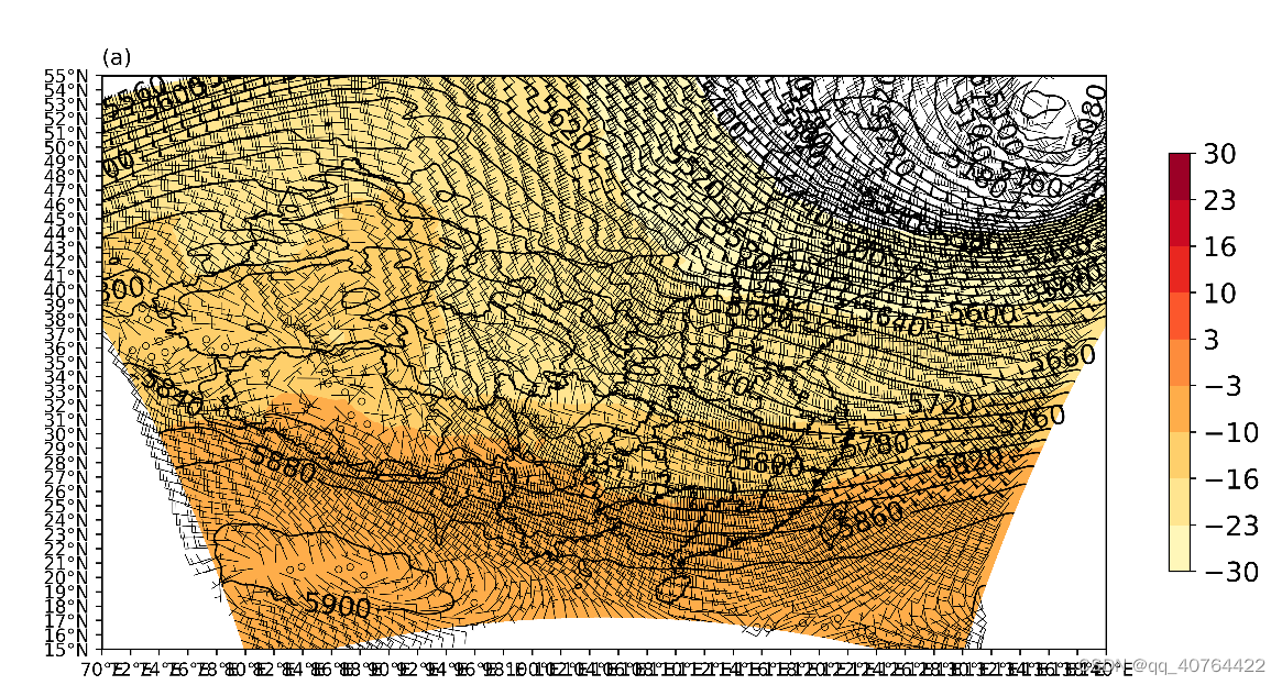

 图片没有细调 大概出来就是这样的 可以根据经纬度进行展示到指定范围呢  需要中国shp文件可以私聊