Principal Component Analysis (PCA) Application and Exploration

Principal Component Analysis (PCA) Application and Exploration

Introduction

In this assignment, I apply Principal Component Analysis (PCA) to a handwritten digits dataset to perform dimensionality reduction and exploratory analysis. PCA is a classical unsupervised linear technique widely used for feature extraction, visualization, and preprocessing in high-dimensional datasets. It works by maximizing variance to construct a lower-dimensional feature space while retaining as much original data information as possible.

The dataset used comes from the UCI repository:

• optdigits.tra: training set with 3823 samples
• optdigits.tes: test set with 1797 samples

Each sample represents an 8×8 image flattened into 64 pixel values and is labeled with a digit (0 to 9), giving a total of 5620 records.

The analysis proceeds as follows:

• Download and prepare the official UCI dataset
• Standardize the data
• Apply PCA with different numbers of principal components (10, 20, 30, 40, 50)
• Visualize the distribution in principal component space
• Compare classification performance before and after PCA (Decision Tree and Random Forest)

Data Preparation & Standardization

Dataset

We use the UCI dataset:

🔗 https://archive.ics.uci.edu/dataset/80/optical+recognition+of+handwritten+digits

We download:

• optdigits.tra (training set)
• optdigits.tes (test set)

Each line contains 65 values: the first 64 are pixel features (range 0–16), and the last is the digit label (0–9).

import pandas as pdtrain_df = pd.read_csv(\"optdigits.tra\", header=None)test_df = pd.read_csv(\"optdigits.tes\", header=None)df = pd.concat([train_df, test_df], ignore_index=True)X = df.iloc[:, :-1].valuesy = df.iloc[:, -1].values

Standardization

Before PCA, we standardize the data using StandardScaler. This ensures each feature contributes equally to variance and avoids dominance by features with larger magnitudes.

from sklearn.preprocessing import StandardScalerscaler = StandardScaler()X_scaled = scaler.fit_transform(X)print(\"Samples:\", X_scaled.shape[0])print(\"Features:\", X_scaled.shape[1])

The 64 features were scaled using StandardScaler, ensuring they have a mean of 0 and a standard deviation of 1. This standardization prepares the data properly for PCA, which is sensitive to the variance of each feature.

PCA Implementation & Principal Components Extraction

Applying PCA

We use sklearn.decomposition.PCA to reduce dimensions with different numbers of principal components: 10, 20, 30, 40, and 50.

from sklearn.decomposition import PCApca_transformed_data = {}explained_variance_ratios = {}component_list = [10, 20, 30, 40, 50]for n in component_list: pca = PCA(n_components=n) X_pca = pca.fit_transform(X_scaled) pca_transformed_data[n] = X_pca explained_variance_ratios[n] = pca.explained_variance_ratio_

Explained Variance Analysis

We calculate cumulative explained variance for all 64 components to determine how many are needed to retain most of the original information.

import matplotlib.pyplot as pltimport numpy as nppca_full = PCA(n_components=64)pca_full.fit(X_scaled)cumulative_variance = np.cumsum(pca_full.explained_variance_ratio_)plt.figure(figsize=(8, 5))plt.plot(range(1, 65), cumulative_variance, marker=\'o\', linestyle=\'-\')plt.title(\'Cumulative Explained Variance vs. Number of Components\')plt.xlabel(\'Number of Principal Components\')plt.ylabel(\'Cumulative Explained Variance Ratio\')plt.grid(True)plt.axhline(y=0.9, color=\'r\', linestyle=\'--\', label=\'90% Variance Threshold\')plt.legend()plt.tight_layout()plt.show()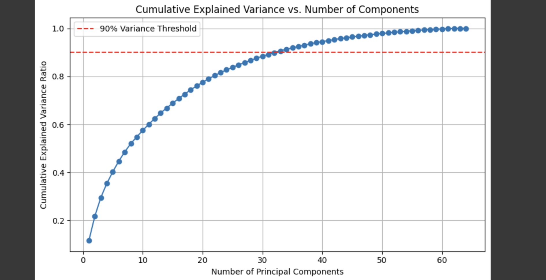

Summary

The plot shows that about 30–40 components are sufficient to retain over 90% of the original variance, striking a good balance between dimensionality and information preservation.

Visualizing PCA Results

We use the first 2 components to plot a 2D visualization of digit classes.

pca_2d = PCA(n_components=2)X_2d = pca_2d.fit_transform(X_scaled)plt.figure(figsize=(8, 6))scatter = plt.scatter(X_2d[:, 0], X_2d[:, 1], c=y, cmap=\'tab10\', alpha=0.7, s=15)plt.title(\"Distribution of Digits in First Two Principal Components\")plt.xlabel(\"Principal Component 1\")plt.ylabel(\"Principal Component 2\")plt.legend(*scatter.legend_elements(), title=\"Digit\")plt.grid(True)plt.tight_layout()plt.show()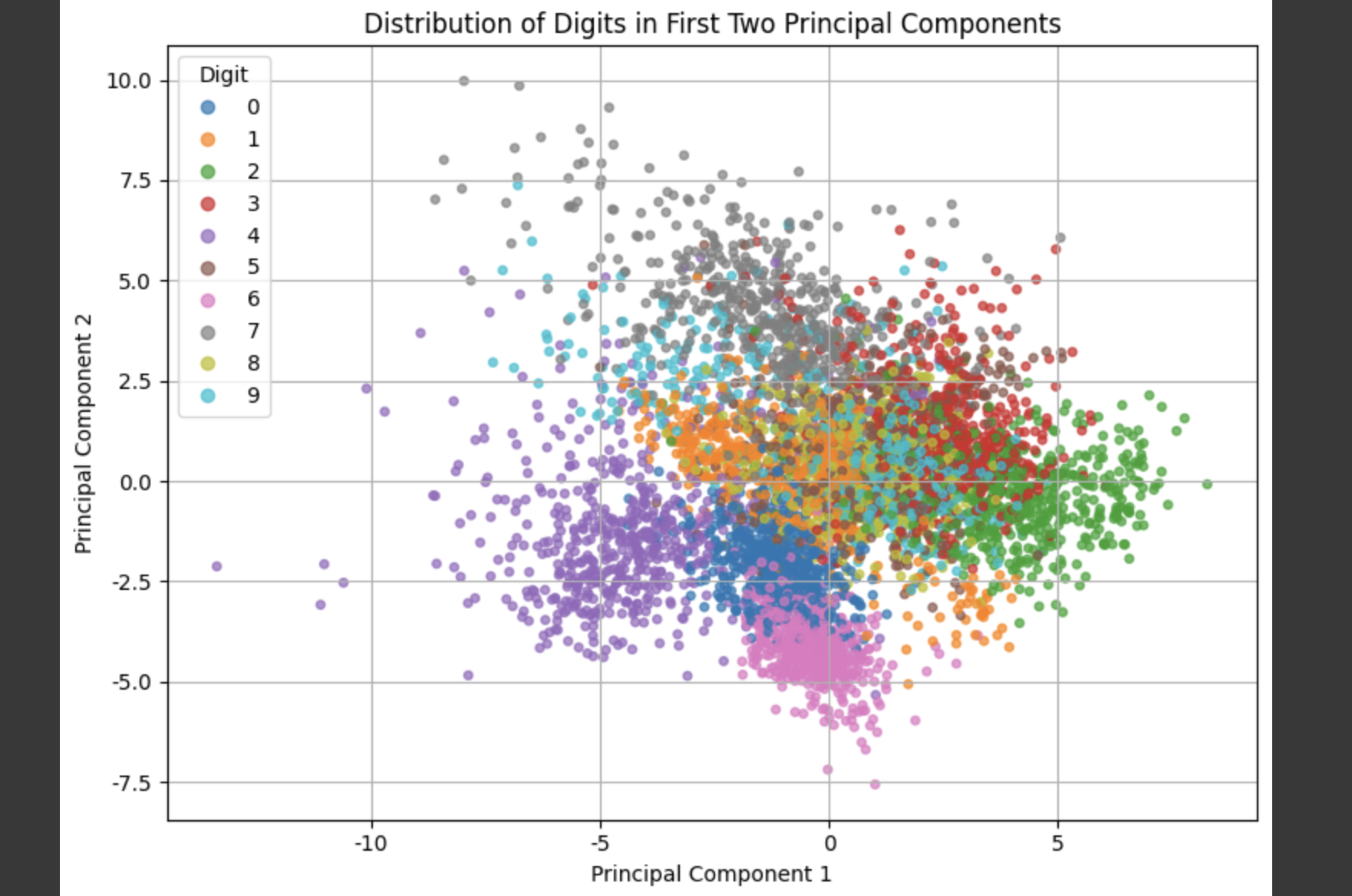

3D Visualization

from mpl_toolkits.mplot3d import Axes3Dpca_3d = PCA(n_components=3)X_3d = pca_3d.fit_transform(X_scaled)fig = plt.figure(figsize=(10, 7))ax = fig.add_subplot(111, projection=\'3d\')scatter = ax.scatter(X_3d[:, 0], X_3d[:, 1], X_3d[:, 2], c=y, cmap=\'tab10\', s=10, alpha=0.6)ax.set_title(\"3D Visualization of First Three Principal Components\")ax.set_xlabel(\"PC1\")ax.set_ylabel(\"PC2\")ax.set_zlabel(\"PC3\")fig.colorbar(scatter)plt.tight_layout()plt.show()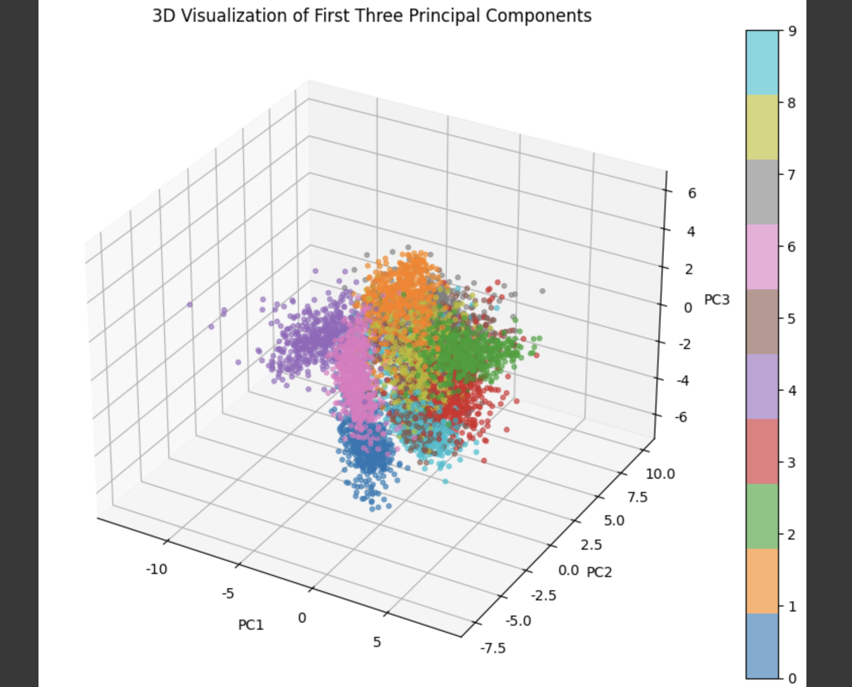

Summary

We successfully applied PCA to reduce the dimensionality of high-dimensional image data and verified its ability to retain most of the important information through visualization and cumulative explained variance analysis. Based on these reduced representations, we will now train classification models to compare their performance across different numbers of principal components.

Classification Model Evaluation with and without PCA

We apply:

• Decision Tree
• Random Forest

On:

1. Original data (64 features)
2. PCA-reduced data (10–50 components)

Dataset Split and Model Setup

from sklearn.model_selection import train_test_splitfrom sklearn.tree import DecisionTreeClassifierfrom sklearn.ensemble import RandomForestClassifierfrom sklearn.metrics import accuracy_scoreX_train, X_test, y_train, y_test = train_test_split( X_scaled, y, test_size=0.2, random_state=42)

Accuracy on Original Data

dt = DecisionTreeClassifier(random_state=42)rf = RandomForestClassifier(random_state=42)dt.fit(X_train, y_train)rf.fit(X_train, y_train)y_pred_dt = dt.predict(X_test)y_pred_rf = rf.predict(X_test)acc_dt_original = accuracy_score(y_test, y_pred_dt)acc_rf_original = accuracy_score(y_test, y_pred_rf)print(f\"Decision Tree Accuracy (Original Data): {acc_dt_original:.4f}\")print(f\"Random Forest Accuracy (Original Data): {acc_rf_original:.4f}\")

Decision Tree Accuracy (Original Data): 0.9004 Random Forest Accuracy (Original Data): 0.9795

PCA Performance Comparison

pca_dt_accuracies = {}pca_rf_accuracies = {}for n in [10, 20, 30, 40, 50]: X_pca = pca_transformed_data[n] X_train_pca, X_test_pca, _, _ = train_test_split( X_pca, y, test_size=0.2, random_state=42 ) dt = DecisionTreeClassifier(random_state=42) rf = RandomForestClassifier(random_state=42) dt.fit(X_train_pca, y_train) rf.fit(X_train_pca, y_train) y_pred_dt = dt.predict(X_test_pca) y_pred_rf = rf.predict(X_test_pca) pca_dt_accuracies[n] = accuracy_score(y_test, y_pred_dt) pca_rf_accuracies[n] = accuracy_score(y_test, y_pred_rf) print(f\"PCA-{n} PCs | Decision Tree Acc: {pca_dt_accuracies[n]:.4f} | Random Forest Acc: {pca_rf_accuracies[n]:.4f}\")

PCA-10 PCs | Decision Tree Acc: 0.8265 | Random Forest Acc: 0.9279 PCA-20 PCs | Decision Tree Acc: 0.8835 | Random Forest Acc: 0.9600 PCA-30 PCs | Decision Tree Acc: 0.8710 | Random Forest Acc: 0.9680 PCA-40 PCs | Decision Tree Acc: 0.8585 | Random Forest Acc: 0.9662 PCA-50 PCs | Decision Tree Acc: 0.8621 | Random Forest Acc: 0.9653

Accuracy Plot

We plotted the classification accuracies under different numbers of principal components to observe how model performance varies with dimensionality reduction.

plt.figure(figsize=(8, 5))plt.plot(pca_dt_accuracies.keys(), pca_dt_accuracies.values(), marker=\'o\', label=\'Decision Tree\')plt.plot(pca_rf_accuracies.keys(), pca_rf_accuracies.values(), marker=\'s\', label=\'Random Forest\')plt.axhline(y=acc_dt_original, color=\'gray\', linestyle=\'--\', label=\'DT (Original)\')plt.axhline(y=acc_rf_original, color=\'black\', linestyle=\'--\', label=\'RF (Original)\')plt.title(\"Accuracy vs. Number of Principal Components\")plt.xlabel(\"Number of Principal Components\")plt.ylabel(\"Accuracy\")plt.legend()plt.grid(True)plt.tight_layout()plt.show()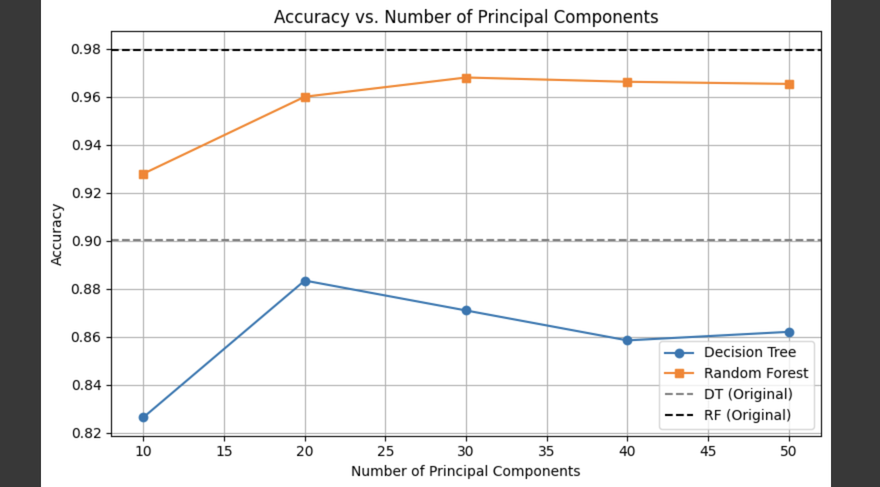

Summary

• On the original (non-reduced) data, Random Forest achieved the highest accuracy, though the model is relatively complex.
• After applying PCA, the accuracy remained relatively stable and high when using between 30 and 50 principal components.
• Decision Trees were more sensitive to dimensionality reduction, with a noticeable drop in performance when using only 10 PCs.
• PCA effectively reduced the number of features while maintaining strong classification performance at lower dimensions, making it a useful method for improving efficiency.

Conclusion

This experiment explored the application of PCA on image data, demonstrating its role in balancing dimensionality reduction with information preservation and classification performance.

Key takeaways:

• Standardization is essential before PCA to ensure fair variance computation.
• Using only 30–40 components can retain over 90% of original variance.
• Random Forest performs well with both original and reduced features.
• Decision Tree is more sensitive to low-dimensional input.
• PCA effectively reduces feature size while maintaining performance — valuable in computationally constrained scenarios.

Full Code

🔗 View Full Code on Google Colab