【DataWhale】快乐学习大模型 | 202507,Task05笔记
前言
今天是Transformer的编码实战阶段,照着示例代码执行一遍吧
embedding
self.tok_embeddings = nn.Embedding(args.vocab_size, args.dim)把token向量转为embedding矩阵(一个token一个embedding向量)
位置编码
为了解决“我喜欢你”和“你喜欢我”结果一致的问题,加入了位置的影响。
小技巧
import pdbpdb.set_trace()在需要打断点的地方加这个,可以暂停python程序进行调试。
Transformer源码和结构图
来自:happy-llm,代码部分做了第2章代码的合并总结,方便本地直接运行。

import torchimport torch.nn as nnimport torch.nn.functional as Fimport math\'\'\'多头自注意力计算模块\'\'\'class MultiHeadAttention(nn.Module): def __init__(self, args, is_causal=False): # 构造函数 # args: 配置对象 super().__init__() # 隐藏层维度必须是头数的整数倍,因为后面我们会将输入拆成头数个矩阵 assert args.dim % args.n_heads == 0 # 模型并行处理大小,默认为1。 model_parallel_size = 1 # 本地计算头数,等于总头数除以模型并行处理大小。 self.n_local_heads = args.n_heads // model_parallel_size # 每个头的维度,等于模型维度除以头的总数。 self.head_dim = args.dim // args.n_heads # Wq, Wk, Wv 参数矩阵,每个参数矩阵为 n_embd x n_embd # 这里通过三个组合矩阵来代替了n个参数矩阵的组合,其逻辑在于矩阵内积再拼接其实等同于拼接矩阵再内积, # 不理解的读者可以自行模拟一下,每一个线性层其实相当于n个参数矩阵的拼接 self.wq = nn.Linear(args.dim, args.n_heads * self.head_dim, bias=False) self.wk = nn.Linear(args.dim, args.n_heads * self.head_dim, bias=False) self.wv = nn.Linear(args.dim, args.n_heads * self.head_dim, bias=False) # 输出权重矩阵,维度为 dim x n_embd(head_dim = n_embeds / n_heads) self.wo = nn.Linear(args.n_heads * self.head_dim, args.dim, bias=False) # 注意力的 dropout self.attn_dropout = nn.Dropout(args.dropout) # 残差连接的 dropout self.resid_dropout = nn.Dropout(args.dropout) self.is_causal = is_causal # 创建一个上三角矩阵,用于遮蔽未来信息 # 注意,因为是多头注意力,Mask 矩阵比之前我们定义的多一个维度 if is_causal: mask = torch.full((1, 1, args.max_seq_len, args.max_seq_len), float(\"-inf\")) mask = torch.triu(mask, diagonal=1) # 注册为模型的缓冲区 self.register_buffer(\"mask\", mask) def forward(self, q: torch.Tensor, k: torch.Tensor, v: torch.Tensor): # 获取批次大小和序列长度,[batch_size, seq_len, dim] bsz, seqlen, _ = q.shape # 计算查询(Q)、键(K)、值(V),输入通过参数矩阵层,维度为 (B, T, n_embed) x (n_embed, n_embed) -> (B, T, n_embed) xq, xk, xv = self.wq(q), self.wk(k), self.wv(v) # 将 Q、K、V 拆分成多头,维度为 (B, T, n_head, C // n_head),然后交换维度,变成 (B, n_head, T, C // n_head) # 因为在注意力计算中我们是取了后两个维度参与计算 # 为什么要先按B*T*n_head*C//n_head展开再互换1、2维度而不是直接按注意力输入展开,是因为view的展开方式是直接把输入全部排开, # 然后按要求构造,可以发现只有上述操作能够实现我们将每个头对应部分取出来的目标 xq = xq.view(bsz, seqlen, self.n_local_heads, self.head_dim) xk = xk.view(bsz, seqlen, self.n_local_heads, self.head_dim) xv = xv.view(bsz, seqlen, self.n_local_heads, self.head_dim) xq = xq.transpose(1, 2) xk = xk.transpose(1, 2) xv = xv.transpose(1, 2) # 注意力计算 # 计算 QK^T / sqrt(d_k),维度为 (B, nh, T, hs) x (B, nh, hs, T) -> (B, nh, T, T) scores = torch.matmul(xq, xk.transpose(2, 3)) / math.sqrt(self.head_dim) # 掩码自注意力必须有注意力掩码 if self.is_causal: assert hasattr(self, \'mask\') # 这里截取到序列长度,因为有些序列可能比 max_seq_len 短 scores = scores + self.mask[:, :, :seqlen, :seqlen] # 计算 softmax,维度为 (B, nh, T, T) scores = F.softmax(scores.float(), dim=-1).type_as(xq) # 做 Dropout scores = self.attn_dropout(scores) # V * Score,维度为(B, nh, T, T) x (B, nh, T, hs) -> (B, nh, T, hs) output = torch.matmul(scores, xv) # 恢复时间维度并合并头。 # 将多头的结果拼接起来, 先交换维度为 (B, T, n_head, C // n_head),再拼接成 (B, T, n_head * C // n_head) # contiguous 函数用于重新开辟一块新内存存储,因为Pytorch设置先transpose再view会报错, # 因为view直接基于底层存储得到,然而transpose并不会改变底层存储,因此需要额外存储 output = output.transpose(1, 2).contiguous().view(bsz, seqlen, -1) # 最终投影回残差流。 output = self.wo(output) output = self.resid_dropout(output) return outputclass MLP(nn.Module): \'\'\'前馈神经网络\'\'\' def __init__(self, dim: int, hidden_dim: int, dropout: float): super().__init__() # 定义第一层线性变换,从输入维度到隐藏维度 self.w1 = nn.Linear(dim, hidden_dim, bias=False) # 定义第二层线性变换,从隐藏维度到输入维度 self.w2 = nn.Linear(hidden_dim, dim, bias=False) # 定义dropout层,用于防止过拟合 self.dropout = nn.Dropout(dropout) def forward(self, x): # 前向传播函数 # 首先,输入x通过第一层线性变换和RELU激活函数 # 然后,结果乘以输入x通过第三层线性变换的结果 # 最后,通过第二层线性变换和dropout层 return self.dropout(self.w2(F.relu(self.w1(x))))class LayerNorm(nn.Module): \'\'\' Layer Norm 层\'\'\' def __init__(self, features, eps=1e-6): super(LayerNorm, self).__init__() # 线性矩阵做映射 self.a_2 = nn.Parameter(torch.ones(features)) self.b_2 = nn.Parameter(torch.zeros(features)) self.eps = eps def forward(self, x): # 在统计每个样本所有维度的值,求均值和方差 mean = x.mean(-1, keepdim=True) # mean: [bsz, max_len, 1] std = x.std(-1, keepdim=True) # std: [bsz, max_len, 1] # 注意这里也在最后一个维度发生了广播 return self.a_2 * (x - mean) / (std + self.eps) + self.b_2class EncoderLayer(nn.Module): \'\'\'Encoder层\'\'\' def __init__(self, args): super().__init__() # 一个 Layer 中有两个 LayerNorm,分别在 Attention 之前和 MLP 之前 self.attention_norm = LayerNorm(args.n_embd) # Encoder 不需要掩码,传入 is_causal=False self.attention = MultiHeadAttention(args, is_causal=False) self.fnn_norm = LayerNorm(args.n_embd) self.feed_forward = MLP(args.n_embd, args.hidden_dim, args.dropout) def forward(self, x): # Layer Norm norm_x = self.attention_norm(x) # 自注意力 h = x + self.attention.forward(norm_x, norm_x, norm_x) # 经过前馈神经网络 out = h + self.feed_forward.forward(self.fnn_norm(h)) return out class Encoder(nn.Module): \'\'\'Encoder 块\'\'\' def __init__(self, args): super(Encoder, self).__init__() # 一个 Encoder 由 N 个 Encoder Layer 组成 self.layers = nn.ModuleList([EncoderLayer(args) for _ in range(args.n_layer)]) self.norm = LayerNorm(args.n_embd) def forward(self, x): \"分别通过 N 层 Encoder Layer\" for layer in self.layers: x = layer(x) return self.norm(x) class DecoderLayer(nn.Module): \'\'\'解码层\'\'\' def __init__(self, args): super().__init__() # 一个 Layer 中有三个 LayerNorm,分别在 Mask Attention 之前、Self Attention 之前和 MLP 之前 self.attention_norm_1 = LayerNorm(args.n_embd) # Decoder 的第一个部分是 Mask Attention,传入 is_causal=True self.mask_attention = MultiHeadAttention(args, is_causal=True) self.attention_norm_2 = LayerNorm(args.n_embd) # Decoder 的第二个部分是 类似于 Encoder 的 Attention,传入 is_causal=False self.attention = MultiHeadAttention(args, is_causal=False) self.ffn_norm = LayerNorm(args.n_embd) # 第三个部分是 MLP self.feed_forward = MLP(args.n_embd, args.hidden_dim, args.dropout) def forward(self, x, enc_out): # Layer Norm norm_x = self.attention_norm_1(x) # 掩码自注意力 x = x + self.mask_attention.forward(norm_x, norm_x, norm_x) # 多头注意力 norm_x = self.attention_norm_2(x) h = x + self.attention.forward(norm_x, enc_out, enc_out) # 经过前馈神经网络 out = h + self.feed_forward.forward(self.ffn_norm(h)) return out class Decoder(nn.Module): \'\'\'解码器\'\'\' def __init__(self, args): super(Decoder, self).__init__() # 一个 Decoder 由 N 个 Decoder Layer 组成 self.layers = nn.ModuleList([DecoderLayer(args) for _ in range(args.n_layer)]) self.norm = LayerNorm(args.n_embd) def forward(self, x, enc_out): \"Pass the input (and mask) through each layer in turn.\" for layer in self.layers: x = layer(x, enc_out) return self.norm(x)class PositionalEncoding(nn.Module): \'\'\'位置编码模块\'\'\' def __init__(self, args): super(PositionalEncoding, self).__init__() # Dropout 层 self.dropout = nn.Dropout(p=args.dropout) # block size 是序列的最大长度 pe = torch.zeros(args.block_size, args.n_embd) position = torch.arange(0, args.block_size).unsqueeze(1) # 计算 theta div_term = torch.exp( torch.arange(0, args.n_embd, 2) * -(math.log(10000.0) / args.n_embd) ) # 分别计算 sin、cos 结果 pe[:, 0::2] = torch.sin(position * div_term) pe[:, 1::2] = torch.cos(position * div_term) pe = pe.unsqueeze(0) self.register_buffer(\"pe\", pe) def forward(self, x): # 将位置编码加到 Embedding 结果上 x = x + self.pe[:, : x.size(1)].requires_grad_(False) return self.dropout(x)class Transformer(nn.Module): \'\'\'整体模型\'\'\' def __init__(self, args): super().__init__() # 必须输入词表大小和 block size assert args.vocab_size is not None assert args.block_size is not None self.args = args self.transformer = nn.ModuleDict(dict( wte = nn.Embedding(args.vocab_size, args.n_embd), wpe = PositionalEncoding(args), drop = nn.Dropout(args.dropout), encoder = Encoder(args), decoder = Decoder(args), )) # 最后的线性层,输入是 n_embd,输出是词表大小 self.lm_head = nn.Linear(args.n_embd, args.vocab_size, bias=False) # 初始化所有的权重 self.apply(self._init_weights) # 查看所有参数的数量 print(\"number of parameters: %.2fM\" % (self.get_num_params()/1e6,)) \'\'\'统计所有参数的数量\'\'\' def get_num_params(self, non_embedding=False): # non_embedding: 是否统计 embedding 的参数 n_params = sum(p.numel() for p in self.parameters()) # 如果不统计 embedding 的参数,就减去 if non_embedding: n_params -= self.transformer.wpe.weight.numel() return n_params \'\'\'初始化权重\'\'\' def _init_weights(self, module): # 线性层和 Embedding 层初始化为正则分布 if isinstance(module, nn.Linear): torch.nn.init.normal_(module.weight, mean=0.0, std=0.02) if module.bias is not None: torch.nn.init.zeros_(module.bias) elif isinstance(module, nn.Embedding): torch.nn.init.normal_(module.weight, mean=0.0, std=0.02) \'\'\'前向计算函数\'\'\' def forward(self, idx, targets=None): # 输入为 idx,维度为 (batch size, sequence length, 1);targets 为目标序列,用于计算 loss device = idx.device b, t = idx.size() assert t <= self.args.block_size, f\"不能计算该序列,该序列长度为 {t}, 最大序列长度只有 {self.args.block_size}\" # 通过 self.transformer # 首先将输入 idx 通过 Embedding 层,得到维度为 (batch size, sequence length, n_embd) print(\"idx\",idx.size()) # 通过 Embedding 层 tok_emb = self.transformer.wte(idx) print(\"tok_emb\",tok_emb.size()) # 然后通过位置编码 pos_emb = self.transformer.wpe(tok_emb) # 再进行 Dropout x = self.transformer.drop(pos_emb) # 然后通过 Encoder print(\"x after wpe:\",x.size()) enc_out = self.transformer.encoder(x) print(\"enc_out:\",enc_out.size()) # 再通过 Decoder x = self.transformer.decoder(x, enc_out) print(\"x after decoder:\",x.size()) if targets is not None: # 训练阶段,如果我们给了 targets,就计算 loss # 先通过最后的 Linear 层,得到维度为 (batch size, sequence length, vocab size) logits = self.lm_head(x) # 再跟 targets 计算交叉熵 loss = F.cross_entropy(logits.view(-1, logits.size(-1)), targets.view(-1), ignore_index=-1) else: # 推理阶段,我们只需要 logits,loss 为 None # 取 -1 是只取序列中的最后一个作为输出 logits = self.lm_head(x[:, [-1], :]) # note: using list [-1] to preserve the time dim loss = None return logits, lossif __name__ == \'__main__\': class Args: vocab_size = 10000 block_size = 128 n_embd = 256 dropout = 0.1 n_layer = 6 n_heads = 8 dim = 256 hidden_dim = 512 dropout = 0.1 max_seq_len = 128 args = Args() model = Transformer(args) print(model) # 训练模型是有target print(\"########## Training ##########\") target = torch.randint(0, args.vocab_size, (2, args.block_size)) logits, loss = model(target, target) print(\"Training logits shape:\", logits.shape) print(\"logits shape:\", logits.shape) print(\"loss:\", loss) # 测试模型的前向计算 print(\"########## Inference ##########\") idx = torch.randint(0, args.vocab_size, (2, args.block_size)) logits, loss = model(idx) print(\"Inference logits shape:\", logits.shape) print(\"logits shape:\", logits.shape) print(\"loss:\", loss)将上面代码保存为 transformer_demo.py 后,直接运行即可
python .\\transformer_demo.py运行结果
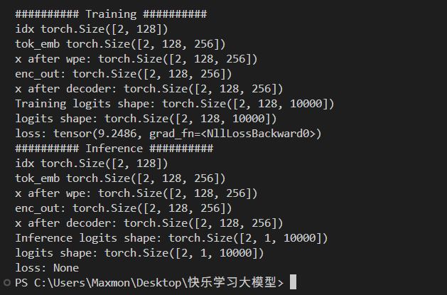
可以看到训练模式下计算了loss(真实GPU训练还会再稍复杂一些)。推理模式下直接推理了下一个的输出,[2,1,10000]中,10000是词表大小,2是batch(如同时2个人在用),1是下一次token。10000中最大的数值最大的位置就是下次概率最大的token。
参考链接
1、happy-llm/docs/chapter2/第二章 Transformer架构.md


