计算机视觉编程基础知识

技术文档

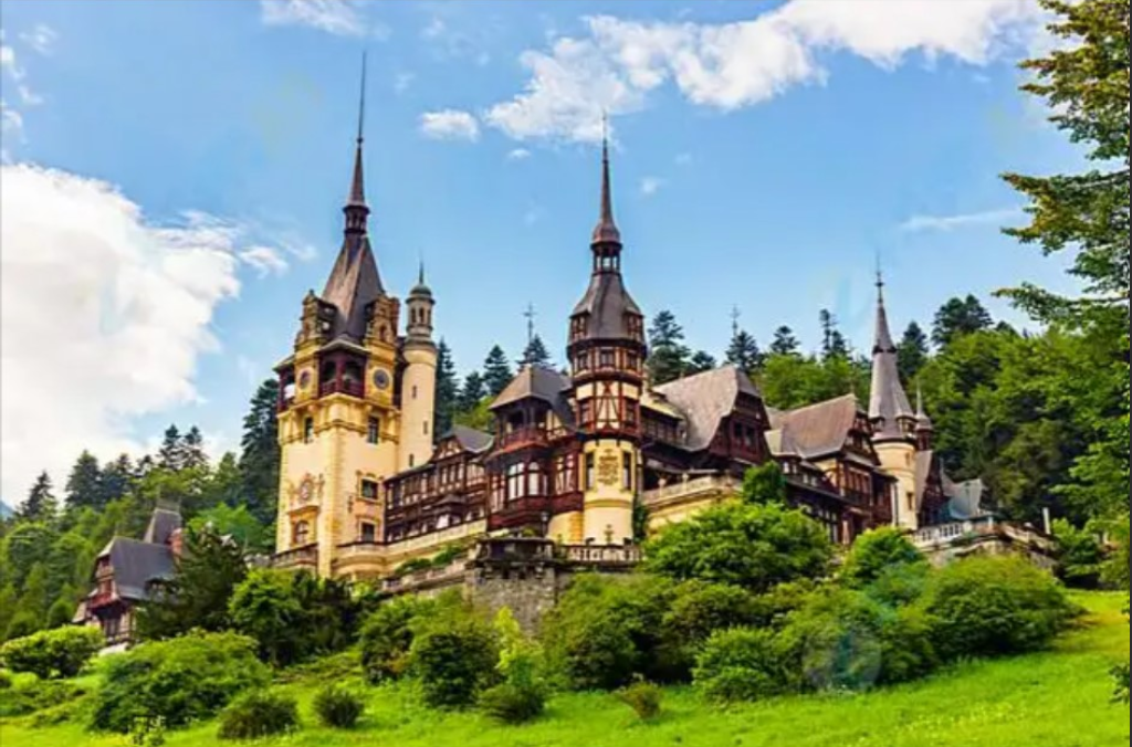
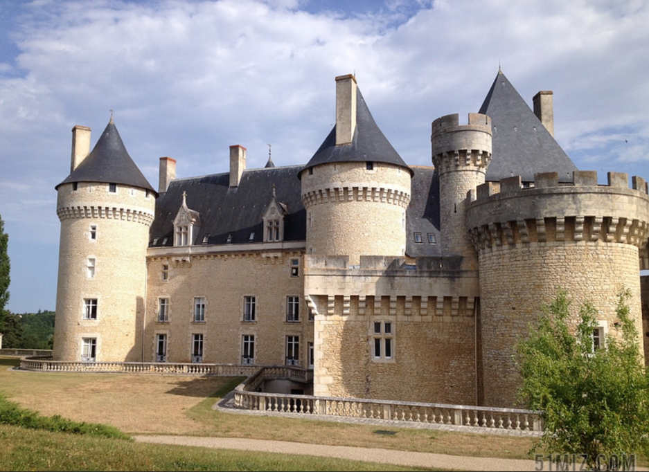
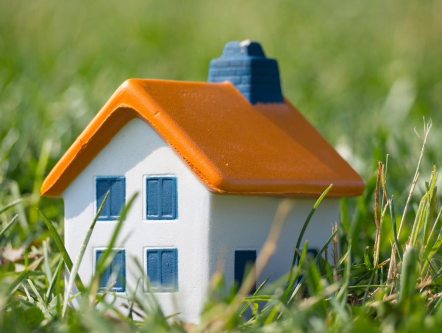
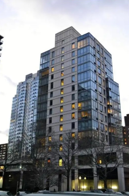
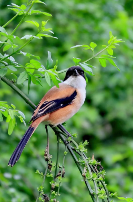
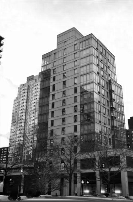
一、本文计算机视觉编程可能用到的图像

二、计算机视觉编程基础知识

三、总结

一、本文计算机视觉编程可能用到的图像

二、计算机视觉编程基础知识

1.numpy库

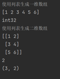
numpy是一个Python中非常基础的用于进行科学计算的库，它的功能包括高维数组计算、线性代数计算、傅里叶变换以及生产伪随机数等。numpy对于scikit-learn来说是至关重要的，因为scikit-learn使用numpy数组形式的数据来进行处理，所以需要把数据都转化成numpy数组的形式，而多维数组也是Numpy的核心功能之一。以下是简单的numpy库的代码展示

import numpyprint(\'使用列表生成一维数组\')data = [1, 2, 3, 4, 5, 6]x = numpy.array(data)print(x) # 打印数组print(x.dtype) # 打印数组元素的类型print(\'使用列表生成二维数组\')data = [[1, 2], [3, 4], [5, 6]]x = numpy.array(data)print(x) # 打印数组print(x.ndim) # 打印数组的维度print(x.shape) # 打印数组各个维度的长度.shape是一个元组

程序运行结果如下：

2.scipy库

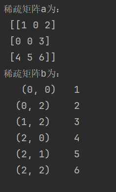
scipy是一个Python中用于进行科学计算的工具集，它有很多功能，如计算统计学分布、信号处理、计算线性代数方程等。scikit-learn需要使用scipy来对算法进行执行，其中用的最多的就是scipy中的sparse函数了。sparse函数用来生成稀疏矩阵，而稀疏矩阵用来存储那些大部分数值位0的数组，这种类型的数组在scikit-learn的实际应用中也非常常见。

下面用实例来展示sparse函数的用法

import numpy as npfrom scipy.sparse import csr_matrixindptr = np.array([0, 2, 3, 6])indices = np.array([0, 2, 2, 0, 1, 2])data = np.array([1, 2, 3, 4, 5, 6])a = csr_matrix((data, indices, indptr), shape=(3, 3)).toarray()print(\'稀疏矩阵a为：\\n\', a)b = csr_matrix(a)print(\'稀疏矩阵b为：\\n\', b)

或者如下写法：

import numpy as npfrom scipy import sparseindptr = np.array([0, 2, 3, 6])indices = np.array([0, 2, 2, 0, 1, 2])data = np.array([1, 2, 3, 4, 5, 6])a = sparse.csr_matrix((data, indices, indptr), shape=(3, 3)).toarray()print(\'稀疏矩阵a为：\\n\', a)b = sparse.csr_matrix(a)print(\'稀疏矩阵b为：\\n\', b)

程序运行结果如下：

3.pandas库

pandas是一个Python中用于进行数据分析的库，它可以生成类似Excel表格式的数据表，而且可以对数据表进行修改操作。pandas还有个强大的功能，它可以从很多不同种类的数据库中提取数据，如SQL数据库、Excel表格甚至CSV文件。pandas还支持在不同的列表中使用不同类型的数据，如整型数据、浮点数或是字符串。下面用一个例子来说明pandas的功能

import pandas as pdfrom pandas import Series, DataFrameprint(\'用一维数组生成Series\')x = Series([1, 2, 3, 4])print(x)print(x.values) # [1, 2, 3, 4]# 默认标签为0到3的序号print(x.index) # RangeIndex(start = 0, stop = 4, step = 1)print(\'指定Series的index\')  # 可将index理解为行索引x = Series([1, 2, 3, 4], index=[\'a\', \'b\', \'d\', \'c\'])print(x)print(x.index)  # Index([u\'a\', u\'b\', u\'d\', u\'c\'], dtype=\'object\')print(x[\'a\']) # 通过行索引来取得元素值：1x[\'d\'] = 6  # 通过行索引来赋值print(x[[\'c\', \'a\', \'d\']]) # 类似于numpy的花式索引

程序运行结果如下：

用一维数组生成Series
0 1
1 2
2 3
3 4
dtype: int64
[1 2 3 4]
RangeIndex(start=0, stop=4, step=1)
指定Series的index
a 1
b 2
d 3
c 4
dtype: int64
Index([\'a\', \'b\', \'d\', \'c\'], dtype=\'object\')
1
c 4
a 1
d 6
dtype: int64

4.图像处理库PIL

PIL（Python Imaging Library，图像处理库）提供了通用的图像处理功能，以及大量有用的基本图像操作。PIL的主要功能定义在Image类中，而Image类定义在同名的Image模块中。使用PIL的功能，一般都是从新建一个Image类的实例开始。新建Image类的实例有多种方法。可以用Image模块的open()函数打开已有的图片档案，也可以处理其他的实例，或者从零开始构建一个实例。

下面实例尝试读入一幅图像

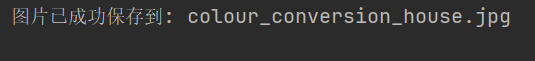
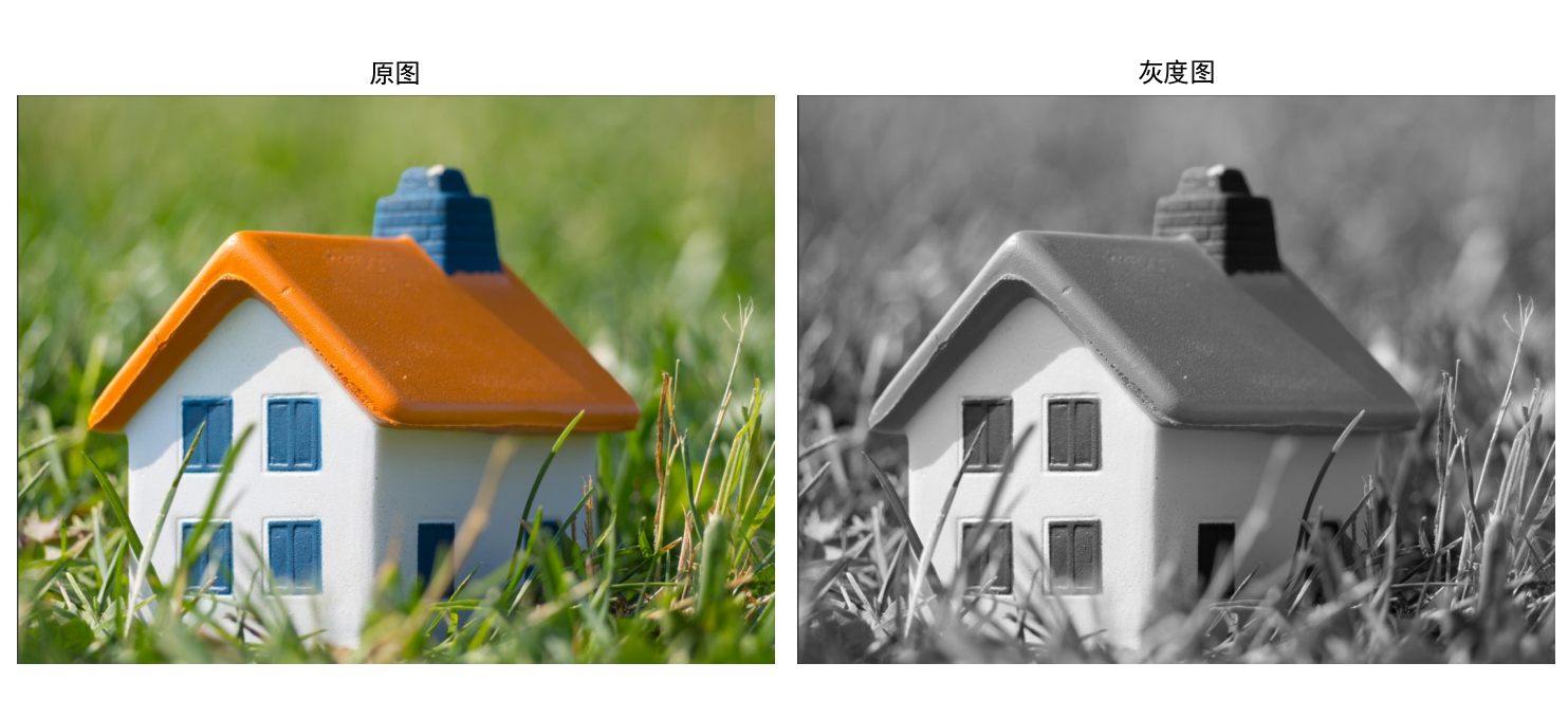
import matplotlib.pyplot as pltfrom PIL import Imagedef display_and_save_image_comparison(original_path, output_path): \"\"\" 显示原图和灰度图的对比并保存结果 参数: original_path: 原始图片路径 output_path: 输出图片路径 \"\"\" # 设置中文字体支持 plt.rcParams[\"font.family\"] = [\"SimHei\"] try: # 创建图像显示窗口 plt.figure(figsize=(10, 5)) # 显示原图 with Image.open(original_path) as img: plt.subplot(121) plt.title(\"原图\") plt.axis(\'off\') plt.imshow(img) # 显示灰度图 with Image.open(original_path) as img: gray_img = img.convert(\'L\') plt.subplot(122) plt.title(\"灰度图\") plt.axis(\'off\') plt.imshow(gray_img, cmap=\'gray\') # 调整布局 plt.tight_layout() # 保存图片 plt.savefig(output_path, dpi=300, bbox_inches=\'tight\') print(f\"图片已成功保存到: {output_path}\") # 显示图片 plt.show() except FileNotFoundError: print(f\"错误：找不到文件 - {original_path}\") except Exception as e: print(f\"发生未知错误: {e}\")if __name__ == \"__main__\": # 设置图片路径 original_image_path = \'house.jpg\' output_image_path = \'colour_conversion_house.jpg\' # 执行图片对比显示和保存 display_and_save_image_comparison(original_image_path, output_image_path)

程序运行结果如下：

5.转换图像格式

对于彩色图像，不管其图像格式是PNG、BMP，还是JPG，在PIL中，使用Image模块的open()函数打开后，返回的图像对象的模式都是RGB。而对于灰度图像，不管其图像格式是PNG、BMP，还是JPG，打开后，其模式都为L。

对于PNG、BMP和JPG彩色图像格式之间的互相转换都可以通过Image模块的open()和save()函数来完成。具体来说，就是在打开这些图像时，PIL会将它们解码为三通道的RGB图像。用户可以基于这个RGB图像，对其进行处理。处理完毕，使用函数save()，可以将处理结果保存成PNG、BMP和JPG中的任何格式。这样也就完成了几种格式之间的转换。同理，其他格式的彩色图像也可以通过这种方式完成转换。当然，对于不同格式的灰度图像，也可以通过类似的途径完成，只是PIL解码后是模式为L的图像。

此处详细介绍一下Image模块的convert()函数，它用于不同模式图像之间的转换。图像的模式转换类型有：

（1）模式为L的灰度图像

（2）模式P为8位彩色图像

（3）模式RGBA为32位彩色图像

（4）模式CMYK位32位彩色图像

（5）模式YCbCr为24位彩色图像

（6）模式I为32位整型灰色图像

（7）模式F为32位浮点灰色图像

模式F与模式L的转换公式一样的，都是RGB转换为灰色值的公式。

使用不同的参数，将当前的图像转换为新的模式，并产生新的图像作为返回值。

实例实现将lena.png图像转换为lena.jpg。

from PIL import Imageimport osdef is_valid_image(img_path): \"\"\"判断文件是否为有效（完整）的图片\"\"\" # 检查文件是否存在 if not os.path.exists(img_path): print(f\"错误：文件不存在 - {img_path}\") return False # 检查文件扩展名 valid_extensions = [\'.jpg\', \'.jpeg\', \'.png\', \'.gif\', \'.bmp\'] ext = os.path.splitext(img_path)[1].lower() if ext not in valid_extensions: print(f\"错误：不支持的文件格式 - {ext}\") return False try: # 尝试打开并加载图像数据 with Image.open(img_path) as img: img.load() # 验证图像数据是否可读取 return True except FileNotFoundError: print(f\"错误：文件不存在 - {img_path}\") except PermissionError: print(f\"错误：没有权限访问 - {img_path}\") except Image.UnidentifiedImageError: print(f\"错误：无法识别的图像格式 - {img_path}\") except (IOError, SyntaxError) as e: print(f\"图片验证失败: {e}\") except Exception as e: print(f\"未知错误: {e}\") return Falsedef transimg(img_path, quality=95, overwrite=False): \"\"\" 转换图片格式为JPG 参数: img_path: 图片路径 quality: JPG质量 (1-95) overwrite: 是否覆盖已存在文件 返回: 成功返回新文件路径，失败返回None \"\"\" if not is_valid_image(img_path): return None # 确保质量参数在有效范围 quality = max(1, min(95, quality)) # 构建输出路径 base_name, _ = os.path.splitext(img_path) output_img_path = f\"{base_name}.jpg\" # 检查文件是否已存在 if os.path.exists(output_img_path) and not overwrite: print(f\"跳过: 文件已存在 - {output_img_path}\") return output_img_path try: print(f\"正在处理: {img_path}\") with Image.open(img_path) as img: # 处理RGBA模式图片（带透明通道） if img.mode == \'RGBA\': background = Image.new(\'RGB\', img.size, (255, 255, 255)) background.paste(img, mask=img.split()[3]) img = background elif img.mode != \'RGB\': img = img.convert(\'RGB\') # 保存为JPG格式 img.save(output_img_path, \'JPEG\', quality=quality) print(f\"成功转换图片: {img_path} -> {output_img_path}\") return output_img_path except FileNotFoundError: print(f\"错误：源文件不存在 - {img_path}\") except PermissionError: print(f\"错误：没有权限写入 - {output_img_path}\") except Exception as e: print(f\"转换失败: {e}\") return Noneif __name__ == \'__main__\': img_path = \'lena.png\' result = transimg(img_path) if result: print(f\"图片已成功转换为: {result}\") else: print(\"图片转换失败\")

程序运行结果如下：

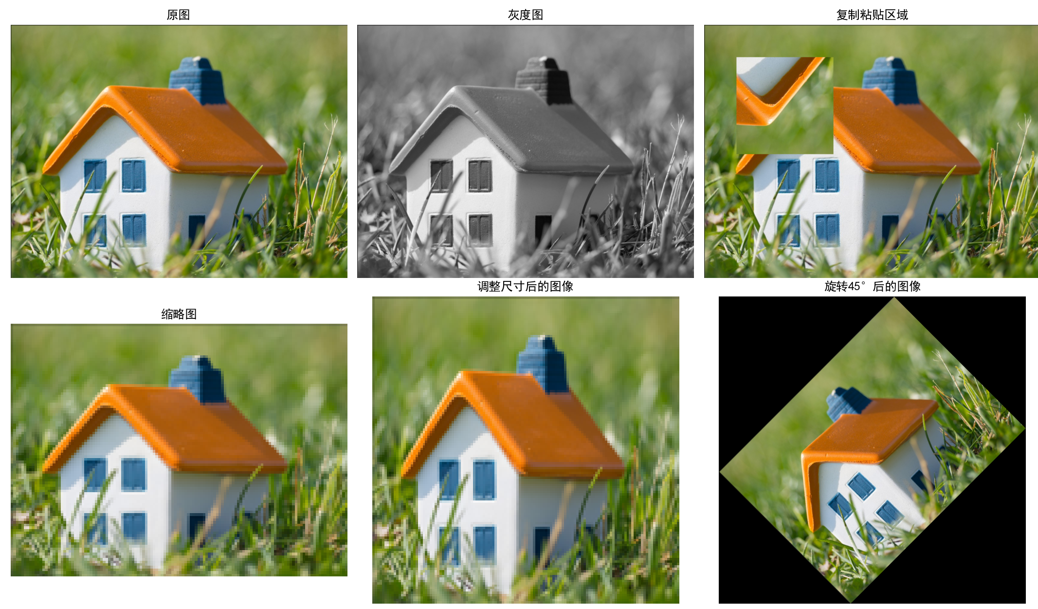
6.图像的基本操作

图像读取与基础信息获取

使用PIL.Image.open()读取图像文件，获取图像的基本属性（模式、尺寸、格式）
这是所有图像处理的基础步骤，用于将数字图像加载到计算机内存中进行后续处理

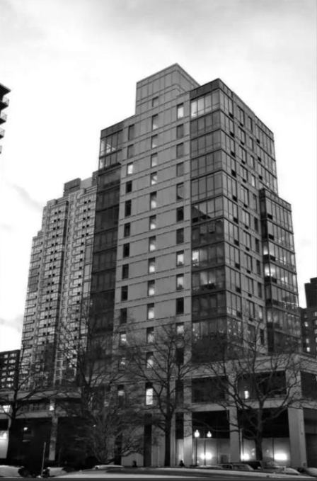
灰度转换

通过convert(\'L\')将彩色图像转换为灰度图
灰度化是计算机视觉中常用的预处理步骤，减少数据维度同时保留关键结构信息，便于后续特征提取

图像裁剪与区域操作

使用crop()方法从原图中提取特定区域（ROI，感兴趣区域）
通过paste()方法将处理后的区域放回原图，实现局部图像修改
结合transpose(Image.ROTATE_180)对裁剪区域进行 180 度旋转
区域操作在目标检测、图像编辑等任务中广泛应用

图像缩放技术

实现了两种缩放方式：
- thumbnail()：保持原图比例生成缩略图（不改变原图）
- resize()：直接调整图像尺寸到指定大小
图像缩放是处理不同分辨率图像的基础技术，在图像金字塔、多尺度分析中常用

图像旋转

使用rotate(45, expand=True)实现图像 45 度旋转
几何变换是计算机视觉的基础操作，用于校正图像角度、适应不同视角等场景

图像可视化与结果展示

利用matplotlib创建多子图布局，对比展示不同处理效果
图像可视化是分析处理结果、调试算法的重要手段

完整Python代码如下：

import matplotlib.pyplot as pltfrom PIL import Imagedef process_image_demo(image_path, output_path): \"\"\" 演示多种图像处理操作并保存结果 参数: image_path: 原始图像路径 output_path: 输出图像路径 \"\"\" # 设置中文字体支持 plt.rcParams[\"font.family\"] = [\"SimHei\"] try: # 创建2x3的子图布局 fig, axes = plt.subplots(2, 3, figsize=(15, 10)) axes = axes.flatten() # 1. 显示原图 with Image.open(image_path) as original_img: print(f\"原图信息: 模式={original_img.mode}, 尺寸={original_img.size}, 格式={original_img.format}\") # 1. 原图 axes[0].set_title(\"原图\") axes[0].axis(\'off\') axes[0].imshow(original_img) # 2. 灰度图 gray_img = original_img.convert(\'L\') axes[1].set_title(\"灰度图\") axes[1].axis(\'off\') axes[1].imshow(gray_img, cmap=\'gray\') # 3. 复制粘贴区域 crop_box = (100, 100, 400, 400) modified_img = original_img.copy() region = modified_img.crop(crop_box) region = region.transpose(Image.ROTATE_180) modified_img.paste(region, crop_box) axes[2].set_title(\"复制粘贴区域\") axes[2].axis(\'off\') axes[2].imshow(modified_img) # 4. 缩略图 (不覆盖原图) thumbnail_img = original_img.copy() thumbnail_size = (128, 128) thumbnail_img.thumbnail(thumbnail_size) print(f\"缩略图尺寸: {thumbnail_img.size}\") axes[3].set_title(\"缩略图\") axes[3].axis(\'off\') axes[3].imshow(thumbnail_img) # 5. 调整尺寸 resized_img = original_img.resize(thumbnail_size) print(f\"调整后尺寸: {resized_img.size}\") axes[4].set_title(\"调整尺寸后的图像\") axes[4].axis(\'off\') axes[4].imshow(resized_img) # 6. 旋转45° rotated_img = original_img.rotate(45, expand=True) axes[5].set_title(\"旋转45°后的图像\") axes[5].axis(\'off\') axes[5].imshow(rotated_img) # 调整布局并保存 plt.tight_layout() plt.savefig(output_path, dpi=300, bbox_inches=\'tight\') print(f\"结果已保存到: {output_path}\") # 显示图像 plt.show() except FileNotFoundError: print(f\"错误：找不到文件 - {image_path}\") except Exception as e: print(f\"发生未知错误: {e}\")if __name__ == \"__main__\": # 设置图片路径 original_image_path = \'house.jpg\' output_image_path = \'Resize_And_Rotate_house.jpg\' # 执行图像处理演示 process_image_demo(original_image_path, output_image_path)

程序运行结果如下：

7.画图、描点和线

图像格式转换

将彩色图像转换为灰度图像（convert(\'L\')），这是视觉任务中常用的预处理步骤，可简化计算同时保留关键结构信息
同时处理和展示彩色与灰度两种版本，便于对比分析

坐标系统与比例计算

采用相对比例计算坐标点（x_ratio和y_ratio），而非固定像素值，确保标注在不同尺寸图像上都能保持合理位置
这种动态坐标计算方法是视觉系统中适应不同分辨率输入的常用策略

图像标注技术

使用标记点（scatter）标记关键位置，模拟特征点检测结果的可视化
通过连接线（plot）展示点之间的关系，类似于目标轮廓标注或特征匹配连线
红色星形标记与蓝色虚线组合形成清晰的视觉对比，符合视觉标注的最佳实践

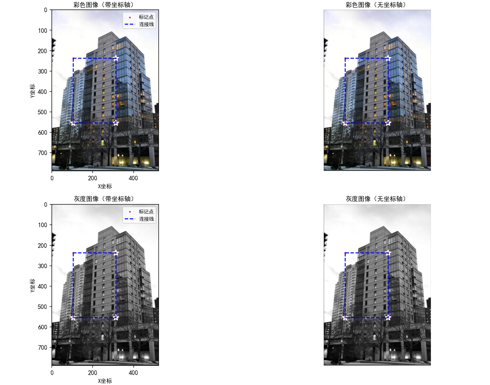
多视图展示

设计 2×2 布局的子图系统，同时展示：
- 带坐标轴的彩色图像（便于精确定位）
- 无坐标轴的彩色图像（专注于视觉效果）
- 带坐标轴的灰度图像（用于分析灰度特征位置）
- 无坐标轴的灰度图像（用于直观观察灰度区域标注）
这种多视图对比是视觉算法调试和结果分析的标准方法

可视化优化

精心调整字体大小、标题位置和子图间距，避免标注元素重叠
合理设置图例位置和标记样式，确保标注信息清晰可读
支持图像保存功能，便于结果归档和分析

用PyLab库绘图的基本颜色格式命令

符号颜色 \'b\' 蓝色 \'g\' 绿色 \'r\' 红色 \'c\' 青色 \'k\' 黑色 \'w\' 白色 \'m\' 品红 \'y\' 黄色

用PyLab库绘图的基本线性格式命令

符号线型 \'-\' 实线 \'--\' 虚线 \'. \' 点线 \'-. \' 点虚线

用PyLab库绘图的基本绘制标记格式命令

符号线型 \'.\' 点 \'s\' 正方形 \'+\' 加号 \'^\'、\'v\'、\'\' 三角形（上下左右） \'o\' 圆圈 \'*\' 星号 ‘×\' 叉号 \'1\'、\'2\'、\'3\'、\'4\' 三叉号（上下左右）

Python代码如下

import matplotlib.pyplot as pltfrom PIL import Imagedef plot_on_image(image_path, output_path=None): \"\"\" 在彩色和灰度图像上绘制点和线，优化布局避免字体重叠 \"\"\" # 设置中文字体支持 plt.rcParams[\"font.family\"] = [\"SimHei\"] plt.rcParams[\'axes.unicode_minus\'] = False # 解决负号显示问题 plt.rcParams[\'axes.titlesize\'] = 10 # 减小标题字体大小 plt.rcParams[\'axes.labelsize\'] = 9 # 减小坐标轴标签字体大小 plt.rcParams[\'legend.fontsize\'] = 8 # 减小图例字体大小 try: # 打开图像并创建灰度版本 with Image.open(image_path) as img: color_img = img.copy() gray_img = img.convert(\'L\') # 转换为灰度图像 img_width, img_height = img.size # 定义要绘制的点和线（根据图像尺寸动态调整坐标，避免超出范围） # 按图像比例计算坐标（避免固定值导致在不同尺寸图像上超出范围） x_ratio = [0.2, 0.2, 0.6, 0.6] # X坐标占图像宽度的比例 y_ratio = [0.3, 0.7, 0.3, 0.7] # Y坐标占图像高度的比例 x_points = [int(x * img_width) for x in x_ratio] y_points = [int(y * img_height) for y in y_ratio] line_indices = [0, 1, 3, 2, 0] # 折线连接顺序 # 创建2x2布局的图像显示窗口，增加垂直间距 plt.figure(figsize=(12, 10)) # 宽12，高10，降低宽高比避免拥挤 # 1. 彩色图像（带坐标轴） plt.subplot(221) plt.imshow(color_img) plt.scatter(x_points, y_points, s=80, marker=\'*\', color=\'red\', edgecolor=\'white\', linewidth=1.5, label=\'标记点\') plt.plot([x_points[i] for i in line_indices],  [y_points[i] for i in line_indices],  \'b--\', linewidth=1.5, label=\'连接线\') plt.title(\"彩色图像（带坐标轴）\", pad=5) # pad=5减小标题与图像间距 plt.xlabel(\"X坐标\") plt.ylabel(\"Y坐标\") plt.legend(loc=\'upper right\') # 固定图例位置，避免遮挡 # 2. 彩色图像（无坐标轴） plt.subplot(222) plt.imshow(color_img) plt.scatter(x_points, y_points, s=80, marker=\'*\', color=\'red\', edgecolor=\'white\', linewidth=1.5) plt.plot([x_points[i] for i in line_indices],  [y_points[i] for i in line_indices],  \'b--\', linewidth=1.5) plt.title(\"彩色图像（无坐标轴）\", pad=5) plt.axis(\'off\') # 3. 灰度图像（带坐标轴） plt.subplot(223) plt.imshow(gray_img, cmap=\'gray\') plt.scatter(x_points, y_points, s=80, marker=\'*\', color=\'red\', edgecolor=\'white\', linewidth=1.5, label=\'标记点\') plt.plot([x_points[i] for i in line_indices],  [y_points[i] for i in line_indices],  \'b--\', linewidth=1.5, label=\'连接线\') plt.title(\"灰度图像（带坐标轴）\", pad=5) plt.xlabel(\"X坐标\") plt.ylabel(\"Y坐标\") plt.legend(loc=\'upper right\') # 4. 灰度图像（无坐标轴） plt.subplot(224) plt.imshow(gray_img, cmap=\'gray\') plt.scatter(x_points, y_points, s=80, marker=\'*\', color=\'red\', edgecolor=\'white\', linewidth=1.5) plt.plot([x_points[i] for i in line_indices],  [y_points[i] for i in line_indices],  \'b--\', linewidth=1.5) plt.title(\"灰度图像（无坐标轴）\", pad=5) plt.axis(\'off\') # 调整子图间距（关键：增加hspace避免标题与下方图像重叠） plt.tight_layout(h_pad=2, w_pad=1) # 垂直间距2，水平间距1 # 保存图像（如果指定了输出路径） if output_path: plt.savefig(output_path, dpi=300, bbox_inches=\'tight\') print(f\"图像已保存到: {output_path}\") # 显示图像 plt.show() except FileNotFoundError: print(f\"错误：找不到文件 - {image_path}\") except Exception as e: print(f\"发生未知错误: {e}\")if __name__ == \"__main__\": original_image_path = \'house2.jpg\' output_image_path = \'color_gray_draw_fixed.jpg\' plot_on_image(original_image_path, output_image_path)

程序运行结果如下：

8.轮廓图与直方图

图像格式转换与预处理

灰度转换技术

通过 PIL.Image.convert(\'L\') 将彩色图像转换为灰度图像（单通道），并通过 np.array() 转为 NumPy 数组以便数值计算。
灰度转换是计算机视觉中最基础的预处理步骤：
- 作用：去除颜色信息干扰，保留亮度（结构）特征，减少数据维度（从 3 通道 RGB 降至 1 通道灰度），降低后续计算复杂度。
- 应用场景：适用于对颜色不敏感的任务（如边缘检测、轮廓分析、OCR 等）。

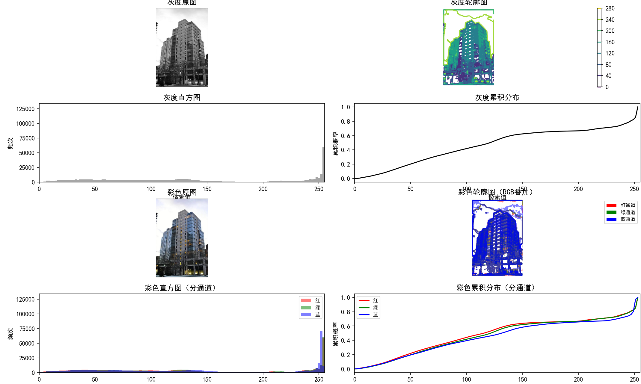
图像结构特征可视化：轮廓图（Contour Plot）

轮廓图是基于像素值变化的结构特征可视化方法，核心原理是通过等高线展示图像中像素值的空间分布差异，本质是对图像亮度梯度的直观呈现。

灰度轮廓图

使用 matplotlib.contour() 对灰度图像的像素值绘制等高线，颜色条（colorbar）表示像素值大小。
作用：突出图像中亮度变化明显的区域（如物体边缘、纹理边界），可视化不同亮度区域的空间分布（例如：图像中的明暗交界线、物体轮廓）。

彩色轮廓图（RGB 通道分离）

对彩色图像的 RGB 三通道分别绘制轮廓（红色对应 R 通道、绿色对应 G 通道、蓝色对应 B 通道），并叠加显示。
作用：单独分析各颜色通道的结构特征，揭示颜色分量的空间分布差异。

像素分布统计分析：直方图（Histogram）

直方图是计算机视觉中像素值统计的核心工具，用于量化图像中不同像素值的出现频次，反映图像的亮度、对比度和颜色分布特征。

灰度直方图

对灰度图像的所有像素值（0-255）进行分箱统计（bins=128），横轴为像素值，纵轴为对应值的出现频次。
作用：
- 判断图像整体亮度（峰值偏左→偏暗，偏右→偏亮）；
- 分析对比度（像素值分布范围窄→低对比度，分布宽→高对比度）；
- 识别噪声或异常区域（如孤立的高 / 低像素值峰值）。

彩色直方图（分通道分析）

对彩色图像的 R、G、B 三通道分别绘制直方图，用红、绿、蓝三色区分。
作用：
- 分析图像的颜色偏向（如 R 通道峰值高→图像偏红，可能为暖色调场景）；
- 检测颜色通道失衡（如某通道像素值集中在低区间→该颜色分量缺失）；
- 为后续颜色校正、图像增强（如白平衡）提供依据。

像素分布累积分析：累积分布函数（CDF）

累积分布函数（CDF）是直方图的衍生统计工具，描述 “像素值小于等于某一阈值的概率”，核心公式为：

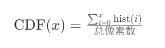
（其中 hist(i) 为像素值 i 的频次）

灰度 CDF

对灰度直方图的频次进行累积求和并归一化（范围 0-1），反映灰度值的累积概率分布。

彩色通道 CDF

分别计算 R、G、B 通道的累积分布函数，用对应颜色曲线展示。

核心作用：

量化图像的对比度特性：CDF 曲线陡峭→像素值集中在窄范围（低对比度）；曲线平缓→像素值分布均匀（高对比度）。
为图像均衡化（Histogram Equalization）提供理论基础：通过调整 CDF 使像素值分布更均匀，提升图像对比度。

多维度特征对比与布局设计

代码通过 4×2 的子图布局，系统展示灰度 / 彩色图像的 “原图 - 轮廓图 - 直方图 - CDF” 四组特征，形成完整的图像特征分析闭环：

子图类型分析目标计算机视觉意义灰度原图提供原始结构参考作为后续分析的基准灰度轮廓图展示亮度变化的空间分布识别物体边缘、区域边界灰度直方图 / CDF 量化灰度值的频次与累积概率判断亮度、对比度，指导灰度增强彩色原图提供原始颜色参考对比颜色与结构的关联彩色轮廓图（RGB 叠加）展示各颜色通道的结构差异分析颜色分量与物体结构的对应关系彩色直方图 / CDF 量化三通道颜色值的分布特征检测颜色偏向，指导颜色校正、白平衡

工程化细节：自适应参数与鲁棒性设计

动态坐标范围：自动计算直方图 Y 轴范围（ylim），基于像素值最大频次加 20% 余量，避免因图像尺寸 / 亮度差异导致的可视化失真。
通道兼容性处理：通过 len(im_color.shape) == 3 判断是否为彩色图像，确保对灰度 / 彩色输入均能稳定处理。

Python代码如下：

import matplotlib.pyplot as pltfrom PIL import Imageimport numpy as np# 设置中文字体支持plt.rcParams[\"font.family\"] = [\"SimHei\"]plt.rcParams[\'axes.unicode_minus\'] = False # 解决负号显示问题def plot_contour_and_histogram(image_path, output_path, bins=128, xlim=(0, 255), ylim=None): \"\"\" 绘制图像的轮廓图和直方图（支持灰度和彩色） 参数: image_path: 输入图像路径 output_path: 输出图像保存路径 bins: 直方图分箱数 xlim: 直方图x轴范围 ylim: 直方图y轴范围（自动计算默认值） \"\"\" try: # 打开图像 with Image.open(image_path) as img: # 转换为灰度图像 im_gray = np.array(img.convert(\'L\')) # 保留彩色图像 im_color = np.array(img) # 计算自动y轴限制（如果未指定） if ylim is None: # 计算所有通道的最大频率，留出20%余量 hist_data = im_gray.flatten() if len(im_color.shape) == 3: # 彩色图像 hist_data = np.concatenate([im_color[:, :, 0].flatten(),im_color[:, :, 1].flatten(),im_color[:, :, 2].flatten()]) _, counts = np.unique(hist_data, return_counts=True) ylim = (0, int(counts.max() * 1.2)) # 留出20%余量 # 创建4x2的子图布局 fig, axes = plt.subplots(4, 2, figsize=(14, 18)) plt.subplots_adjust(hspace=0.3, wspace=0.2) # 调整子图间距 # -------------------- 灰度图像部分 -------------------- # 灰度原图 axes[0, 0].imshow(im_gray, cmap=\'gray\') axes[0, 0].set_title(\'灰度原图\') axes[0, 0].axis(\'off\') # 灰度轮廓图 contour = axes[0, 1].contour(im_gray, origin=\'image\', cmap=\'viridis\') axes[0, 1].set_title(\'灰度轮廓图\') axes[0, 1].axis(\'equal\') axes[0, 1].axis(\'off\') plt.colorbar(contour, ax=axes[0, 1]) # 添加颜色条 # 灰度直方图 axes[1, 0].hist(im_gray.flatten(), bins=bins, color=\'gray\', alpha=0.7) axes[1, 0].set_title(\'灰度直方图\') axes[1, 0].set_xlim(xlim) axes[1, 0].set_ylim(ylim) axes[1, 0].set_xlabel(\'像素值\') axes[1, 0].set_ylabel(\'频次\') # 灰度累积分布函数 hist, bins = np.histogram(im_gray.flatten(), bins=bins, density=True) cdf = hist.cumsum() cdf = cdf / cdf[-1] # 归一化 axes[1, 1].plot(bins[:-1], cdf, \'k-\') axes[1, 1].set_title(\'灰度累积分布\') axes[1, 1].set_xlim(xlim) axes[1, 1].set_xlabel(\'像素值\') axes[1, 1].set_ylabel(\'累积概率\') # -------------------- 彩色图像部分 -------------------- # 彩色原图 axes[2, 0].imshow(im_color) axes[2, 0].set_title(\'彩色原图\') axes[2, 0].axis(\'off\') # 彩色轮廓图（合并显示） if len(im_color.shape) == 3: # 确保是彩色图像 # 分别绘制RGB通道轮廓 r_contour = axes[2, 1].contour(im_color[:, :, 0], levels=5, origin=\'image\', colors=\'red\', alpha=0.5) g_contour = axes[2, 1].contour(im_color[:, :, 1], levels=5, origin=\'image\', colors=\'green\', alpha=0.5) b_contour = axes[2, 1].contour(im_color[:, :, 2], levels=5, origin=\'image\', colors=\'blue\', alpha=0.5) axes[2, 1].set_title(\'彩色轮廓图（RGB叠加）\') axes[2, 1].axis(\'equal\') axes[2, 1].axis(\'off\') # 添加颜色条 r_proxy = plt.Rectangle((0, 0), 1, 1, fc=\'red\') g_proxy = plt.Rectangle((0, 0), 1, 1, fc=\'green\') b_proxy = plt.Rectangle((0, 0), 1, 1, fc=\'blue\') axes[2, 1].legend([r_proxy, g_proxy, b_proxy], [\'红通道\', \'绿通道\', \'蓝通道\'], loc=\'upper right\', fontsize=8) # 彩色直方图（分通道） if len(im_color.shape) == 3: axes[3, 0].hist(im_color[:, :, 0].flatten(), bins=bins, color=\'red\', alpha=0.5, label=\'红\') axes[3, 0].hist(im_color[:, :, 1].flatten(), bins=bins, color=\'green\', alpha=0.5, label=\'绿\') axes[3, 0].hist(im_color[:, :, 2].flatten(), bins=bins, color=\'blue\', alpha=0.5, label=\'蓝\') axes[3, 0].set_title(\'彩色直方图（分通道）\') axes[3, 0].set_xlim(xlim) axes[3, 0].set_ylim(ylim) axes[3, 0].set_xlabel(\'像素值\') axes[3, 0].set_ylabel(\'频次\') axes[3, 0].legend(fontsize=8) # 彩色累积分布函数（分通道） if len(im_color.shape) == 3: # 红色通道 hist_r, bins_r = np.histogram(im_color[:, :, 0].flatten(), bins=bins, density=True) cdf_r = hist_r.cumsum() cdf_r = cdf_r / cdf_r[-1] # 绿色通道 hist_g, bins_g = np.histogram(im_color[:, :, 1].flatten(), bins=bins, density=True) cdf_g = hist_g.cumsum() cdf_g = cdf_g / cdf_g[-1] # 蓝色通道 hist_b, bins_b = np.histogram(im_color[:, :, 2].flatten(), bins=bins, density=True) cdf_b = hist_b.cumsum() cdf_b = cdf_b / cdf_b[-1] # 绘制累积分布 axes[3, 1].plot(bins_r[:-1], cdf_r, \'r-\', label=\'红\') axes[3, 1].plot(bins_g[:-1], cdf_g, \'g-\', label=\'绿\') axes[3, 1].plot(bins_b[:-1], cdf_b, \'b-\', label=\'蓝\') axes[3, 1].set_title(\'彩色累积分布（分通道）\') axes[3, 1].set_xlim(xlim) axes[3, 1].set_xlabel(\'像素值\') axes[3, 1].set_ylabel(\'累积概率\') axes[3, 1].legend(fontsize=8) # 调整布局并保存 plt.tight_layout() plt.savefig(output_path, dpi=300, bbox_inches=\'tight\') print(f\"结果已保存至: {output_path}\") plt.show() except FileNotFoundError: print(f\"错误：未找到图像文件 - {image_path}\") except Exception as e: print(f\"处理出错: {e}\")if __name__ == \"__main__\": # 配置路径和参数 input_img = \"house2.jpg\" output_img = \"color_contour_histogram.jpg\" # 调用函数 plot_contour_and_histogram(input_img, output_img)

程序运行结果如下：

9.交互式标注

图像格式处理与显示优化

灰度图像的真正转换（而非视觉效果）

通过 PIL.Image.convert(\'L\') 将彩色图像转换为单通道灰度图像（像素值范围 0-255），而非仅通过 matplotlib 的 cmap=\'gray\' 进行视觉上的灰度显示。
技术意义：确保后续处理（如坐标映射、特征提取）基于真实的灰度数据，避免彩色通道干扰，符合计算机视觉中 “灰度图简化计算” 的预处理逻辑。

彩色与灰度图像的差异化显示

彩色图像直接以 RGB 三通道数组显示，保留原始颜色信息；灰度图像通过 cmap=\'gray\' 确保视觉上的灰度呈现。
应用价值：满足不同场景的标注需求 —— 彩色图适合依赖颜色特征的标记（如特定颜色物体），灰度图适合依赖结构特征的标记（如边缘、角点）。

交互式坐标获取：用户驱动的特征点标记

代码的核心功能是通过 matplotlib.pyplot.ginput() 实现人机交互的坐标采集，这是计算机视觉中获取 “地面真值”（Ground Truth）的常用手段。

交互式点采集机制

plt.ginput(num_points, timeout=30) 函数监听用户鼠标点击，获取点击位置的像素坐标（X, Y），支持指定采集数量（num_points）和超时时间（30 秒）。
技术本质：将用户的物理交互（鼠标点击）映射为图像的像素坐标系统，建立 “视觉感知” 到 “数值坐标” 的桥梁。

坐标的精准性与应用场景

获取的坐标直接对应图像的像素位置（例如点击图像中某物体的顶点，返回其在图像矩阵中的列索引 X 和行索引 Y）。
典型应用：
- 手动标记特征点（如用于图像配准的对应点对）；
- 定义感兴趣区域（ROI）的顶点（如标记物体边界框的角点）；
- 校准图像（如标记棋盘格角点用于相机内参计算）。

标注可视化与用户体验优化

为确保标记结果清晰可辨，代码设计了针对性的可视化策略，符合计算机视觉标注工具的通用设计原则：

多样式标记与区分

使用不同形状（markers = [\'o\', \'s\', \'^\', \'D\', \'*\']）和颜色（colors = [\'red\', \'blue\', \'green\']）区分多个标记点，避免混淆。
关键优化：为标记点添加白色边缘（edgecolor=\'white\'）和半透明效果（alpha=0.8），确保在复杂背景（如灰度图暗区、彩色图高饱和区域）中依然醒目。

坐标文本标注

通过 plt.text() 在每个点旁添加编号（如 “点 1”“点 2”），并使用白色半透明背景（bbox=dict(facecolor=\'white\', alpha=0.7)）增强可读性。
价值：便于后续对标记点的索引和引用（如在结果分析中区分不同功能的点）。

鲁棒性设计：异常处理与用户反馈

代码通过异常捕获和状态提示，确保交互过程的稳定性，符合工程化视觉工具的要求：

错误处理机制

捕获 FileNotFoundError 处理图像文件不存在的问题，避免程序崩溃；
通用异常捕获（Exception as e）处理点击超时、图像格式错误等意外情况。

用户引导与结果反馈

实时打印提示信息（如 “请单击 3 个点，完成后关闭窗口”），指导用户操作；
输出采集结果（如 “点 1：(x, y)”），明确标记坐标的数值，便于后续使用（如复制到其他算法中）。

Python代码如下：

import matplotlib.pyplot as pltfrom PIL import Imageimport numpy as npdef get_clicked_points(image_path, num_points=3, is_gray=False): \"\"\" 显示图像（支持真正的灰度转换）并获取用户单击的点坐标，同时进行标注 参数: image_path: 图像路径 num_points: 需要获取的点数量 is_gray: 是否将图像真正转换为单通道灰度图（而非仅用灰度配色） 返回: 点坐标列表，每个元素为(x, y)元组 \"\"\" # 设置中文字体，避免中文乱码 plt.rcParams[\"font.family\"] = [\"SimHei\"] plt.rcParams[\'axes.unicode_minus\'] = False # 解决负号显示问题 try: # 安全打开图像并处理 with Image.open(image_path) as img: # 关键修改：真正将图像转换为单通道灰度图（而非仅改变显示方式） if is_gray: img = img.convert(\'L\') # 转换为单通道灰度图（像素值0-255） im_array = np.array(img) # 转换为数组 # 创建画布 plt.figure(figsize=(8, 6)) # 显示图像（根据图像类型选择显示方式） if is_gray: # 单通道灰度图必须用cmap=\'gray\'，否则会被自动上色 plt.imshow(im_array, cmap=\'gray\') plt.title(f\"灰度图像 - 请单击{num_points}个点\", pad=10) else: # 彩色图像直接显示（三通道） plt.imshow(im_array) plt.title(f\"彩色图像 - 请单击{num_points}个点\", pad=10) # 坐标轴设置 plt.axis(\'on\') plt.xlabel(\"X坐标\") plt.ylabel(\"Y坐标\") # 获取用户点击的点 print(f\"提示：在{\'灰度\' if is_gray else \'彩色\'}图像上单击{num_points}个点，完成后关闭窗口...\") points = plt.ginput(num_points, timeout=30) # 30秒超时 # 标注点（不同点用不同样式，确保在灰度图上清晰） if points: markers = [\'o\', \'s\', \'^\', \'D\', \'*\'] # 标记样式 colors = [\'red\', \'blue\', \'green\', \'purple\', \'orange\'] # 标记颜色 for i, (x, y) in enumerate(points):  marker = markers[i % len(markers)]  color = colors[i % len(colors)]  # 绘制带白边的点（在灰度图上更醒目）  plt.scatter(x, y, s=100, marker=marker, color=color, edgecolor=\'white\', linewidth=2, alpha=0.8)  # 标注点编号  plt.text(x + 5, y + 5, f\"点{i + 1}\", fontsize=12, bbox=dict(facecolor=\'white\', alpha=0.7, pad=2)) # 显示标注后暂停，再关闭窗口 plt.draw() plt.pause(1) plt.close() # 输出结果 if len(points) == num_points: print(f\"{\'灰度\' if is_gray else \'彩色\'}图像成功获取{num_points}个点：\") for i, (x, y) in enumerate(points, 1):  print(f\"点{i}：({x}, {y})\") return points else: print(f\"{\'灰度\' if is_gray else \'彩色\'}图像未获取足够的点（仅{len(points)}个）\") return None except FileNotFoundError: print(f\"错误：未找到图像文件 - {image_path}\") return None except Exception as e: print(f\"操作出错：{e}\") return Noneif __name__ == \"__main__\": image_path = \"house2.jpg\" # 先处理彩色图像 print(\"\\n===== 处理彩色图像 =====\") color_points = get_clicked_points(image_path, 3, is_gray=False) # 再处理灰度图像（真正转换为单通道） print(\"\\n===== 处理灰度图像 =====\") gray_points = get_clicked_points(image_path, 3, is_gray=True)

程序运行结果如下：

===== 处理彩色图像 =====
提示：在彩色图像上单击3个点，完成后关闭窗口...
彩色图像成功获取3个点：
点1：(225.09090909090907, 136.29653679653677)
点2：(361.88744588744584, 134.58658008658006)
点3：(481.5844155844156, 336.36147186147184)

===== 处理灰度图像 =====
提示：在灰度图像上单击3个点，完成后关闭窗口...
灰度图像成功获取3个点：
点1：(170.37229437229433, 213.24458874458867)
点2：(361.88744588744584, 127.7467532467532)
点3：(447.3852813852813, 220.08441558441552)

10.图像处理

数字图像的加载与数据结构解析

在计算机视觉中，数字图像本质上是像素值组成的多维数组，代码首先通过PIL和NumPy完成图像的加载与数据格式转换，揭示图像的底层存储逻辑。

彩色图像的 RGB 数组表示

通过Image.open()加载图像后，用np.array()将其转换为 NumPy 数组（rgb_array），得到形状为(高度, 宽度, 3)的三维数组。
- 第一维度：图像高度（像素行数）；
- 第二维度：图像宽度（像素列数）；
- 第三维度：RGB 三通道（分别对应红色、绿色、蓝色分量）。
数据类型：通常为uint8（无符号 8 位整数），像素值范围0-255，这是数字图像的标准存储格式（平衡精度与存储空间）。

关键信息输出

代码打印图像的形状、数据类型和像素值范围，直观展示：
- 图像的空间尺寸（高度 × 宽度）；
- 数据存储精度（uint8确保每个通道像素用 1 字节存储）；
- 亮度分布范围（如像素值集中在低区间说明图像偏暗）。

RGB 通道分离：颜色成分的独立分析

彩色图像的颜色信息由红（R）、绿（G）、蓝（B）三通道叠加而成，通道分离是颜色特征分析的基础技术，代码通过数组切片实现各通道的提取与分析。

通道分离方法

利用 NumPy 数组的索引功能拆分通道：
- 红色通道：r_channel = rgb_array[:, :, 0]（取第三维度的第 0 个元素）；
- 绿色通道：g_channel = rgb_array[:, :, 1]（取第三维度的第 1 个元素）；
- 蓝色通道：b_channel = rgb_array[:, :, 2]（取第三维度的第 2 个元素）。
每个通道均为二维数组（高度×宽度），像素值范围仍为0-255，表示该颜色分量的强度。

通道特征分析

代码计算并输出各通道的关键统计量：
- 像素值范围：反映该颜色分量的动态范围（如红色通道0-255表示红色分量完整，若范围0-50则红色缺失）；
- 均值：反映该颜色的整体强度（如绿色通道均值高说明图像偏绿，可能为自然场景；红色通道均值高可能为暖色调场景）。
应用价值：通道分析是颜色校正、图像增强（如对比度调整）、目标检测（如基于颜色的区域分割）的前提。

灰度转换：从彩色到单通道的降维

灰度转换是计算机视觉中简化图像数据的核心预处理步骤，通过将三通道彩色图像转为单通道灰度图像，保留结构信息的同时降低计算复杂度。

灰度转换方法

代码使用img.convert(\'L\')实现转换（\'L\'是 PIL 库中灰度模式的标识），并转为float32类型便于后续数值计算。
转换原理：基于人眼对不同颜色的敏感度加权计算，标准公式为：
Gray=0.299×R+0.587×G+0.114×B
（人眼对绿色最敏感，权重最高；对蓝色最不敏感，权重最低）。

灰度图像的特征分析

灰度图像为二维数组（高度×宽度），像素值范围0-255（转为float32后保留精度）。
代码输出灰度图像的均值和范围，用于判断：
- 整体亮度（均值高→偏亮，均值低→偏暗）；
- 对比度（范围窄→低对比度；范围宽→高对比度）。

通道图像保存：可视化验证

代码将分离的 RGB 通道和灰度图像保存为独立文件（如red_channel_house2.jpg），通过可视化直观验证通道分离的效果：

红色通道图像中，红色物体区域会呈现高亮，其他区域偏暗；
绿色通道图像中，绿色物体区域会突出显示；
蓝色通道图像中，蓝色物体区域会更清晰；
灰度图像则仅保留亮度信息，无颜色干扰，便于观察物体的轮廓和纹理。

Python代码如下：

import numpy as npfrom PIL import Imagetry: # 打开图像并获取RGB数组 with Image.open(\'house2.jpg\') as img: # 保存原始彩色图像 rgb_array = np.array(img) # 转换为灰度图像并转为浮点类型 gray_array = np.array(img.convert(\'L\'), dtype=np.float32) # 分离RGB三个通道 r_channel = rgb_array[:, :, 0] # 红色通道 g_channel = rgb_array[:, :, 1] # 绿色通道 b_channel = rgb_array[:, :, 2] # 蓝色通道 # 输出原始彩色图像信息 print(\"=\" * 50) print(f\"原始彩色RGB图像信息:\") print(f\" 形状: {rgb_array.shape} (高度, 宽度, 通道数)\") print(f\" 数据类型: {rgb_array.dtype}\") print(f\" 像素值范围: {rgb_array.min()} - {rgb_array.max()}\") print(\"=\" * 50) # 输出各颜色通道信息 print(\"\\n各颜色通道详细信息:\") print(f\" 红色通道 - 像素范围: {r_channel.min()} - {r_channel.max()}, 均值: {r_channel.mean():.1f}\") print(f\" 绿色通道 - 像素范围: {g_channel.min()} - {g_channel.max()}, 均值: {g_channel.mean():.1f}\") print(f\" 蓝色通道 - 像素范围: {b_channel.min()} - {b_channel.max()}, 均值: {b_channel.mean():.1f}\") print(\"=\" * 50) # 输出灰度图像信息 print(\"\\n灰度图像信息:\") print(f\" 形状: {gray_array.shape} (高度, 宽度)\") print(f\" 数据类型: {gray_array.dtype}\") print(f\" 像素值范围: {gray_array.min():.1f} - {gray_array.max():.1f}\") print(f\" 像素均值: {gray_array.mean():.1f}\") print(\"=\" * 50) # 保存分离的通道图像（可选） save_channels = True if save_channels: Image.fromarray(r_channel).save(\'red_channel_house2.jpg\') Image.fromarray(g_channel).save(\'green_channel_house2.jpg\') Image.fromarray(b_channel).save(\'blue_channel_house2.jpg\') Image.fromarray(np.uint8(gray_array)).save(\'gray_channel_house2.jpg\') print(\"已保存各通道图像（红、绿、蓝、灰度）\")except FileNotFoundError: print(\"错误：找不到图像文件 \'house2.jpg\'\")except Exception as e: print(f\"处理图像时出错: {e}\")

程序运行结果如下：

==================================================
原始彩色RGB图像信息:
形状: (790, 523, 3) (高度, 宽度, 通道数)
数据类型: uint8
像素值范围: 0 - 255
==================================================

各颜色通道详细信息:
红色通道 - 像素范围: 0 - 255, 均值: 134.8
绿色通道 - 像素范围: 0 - 255, 均值: 138.1
蓝色通道 - 像素范围: 0 - 255, 均值: 142.8
==================================================

灰度图像信息:
形状: (790, 523) (高度, 宽度)
数据类型: float32
像素值范围: 0.0 - 255.0
像素均值: 137.7
==================================================
已保存各通道图像（红、绿、蓝、灰度）

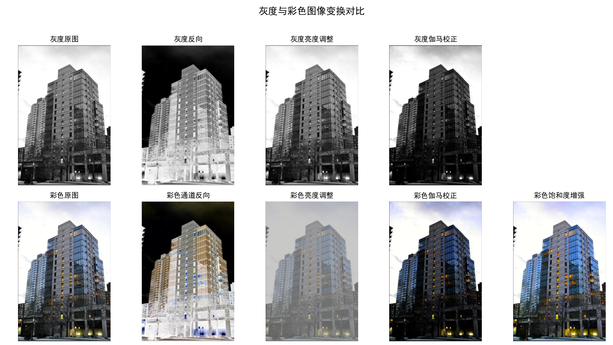
11.灰度与彩色图像变换

图像变换的底层逻辑：点运算（Pixel-wise Operation）

代码中所有变换均属于点运算（仅依赖单个像素的原始值，不涉及邻域像素），是图像处理中最基础的操作类型。其核心逻辑是通过数学函数对每个像素值进行映射（输入像素值→输出像素值），实现图像视觉特征的调整。点运算的优势是计算高效，可批量处理所有像素，广泛用于图像预处理或增强。

灰度图像变换：单通道像素值调整

灰度图像（单通道，像素值 0-255）的变换聚焦于亮度和对比度优化，代码实现了三种经典变换：

（1）灰度反向（Gray Inversion）

原理：通过 gray_invert = 255 - gray_array 实现，每个像素值被其补值（255 减去原始值）替代。
效果：类似 “负片” 效果，暗部变亮、亮部变暗。
应用：增强暗区域细节（如夜景中隐藏的细节）、艺术效果处理，或作为某些特征提取算法的预处理步骤（如边缘检测前的对比度反转）。

（2）灰度亮度调整（Brightness Adjustment）

原理：通过线性映射公式 gray_brightness = np.uint8((100.0/255)*gray_array + 100) 将原始像素值（0-255）缩放到 100-200 范围。
本质：线性点运算 y = a*x + b（其中 a=100/255≈0.39，b=100），通过调整斜率 a 和截距 b 改变整体亮度。
效果：图像整体亮度提升（像素值整体上移），避免原始图像过暗的问题。
应用：校正低光照图像的亮度不足，或统一不同光照条件下图像的亮度水平。

（3）灰度伽马校正（Gamma Correction）

原理：通过非线性映射 gray_gamma = np.uint8(255.0 * (gray_array / 255.0) **2) 实现，本质是伽马变换 y = 255*(x/255)^γ（此处 γ=2）。
-** 特性 **：
- 当 γ>1 时，图像变暗，暗部细节被压缩，亮部对比度增强；
- 当 γ<1 时，图像变亮，亮部细节被压缩，暗部对比度增强。
  -** 应用 **：校正显示器等设备的非线性亮度响应（设备通常存在 γ≈2.2 的非线性），或增强特定亮度区域的细节（如暗部纹理）。

彩色图像变换：多通道协同调整

彩色图像（RGB 三通道）的变换不仅涉及亮度，还包括颜色饱和度等特征，代码实现了四种针对性变换：

（1）彩色通道反向（Color Inversion）

原理：通过 color_invert = 255 - rgb_array 对 RGB 三通道同时执行反向操作，每个通道的像素值均取补值。
效果：类似彩色负片，红色变为青色、绿色变为品红色、蓝色变为黄色（RGB 互补色原理）。
特点：保留颜色通道间的相对关系，仅反转亮度，常用于艺术创作或特殊场景增强（如医学图像的负片查看）。

（2）彩色亮度调整（Color Brightness Adjustment）

原理：与灰度亮度调整逻辑一致，通过线性映射 color_brightness = np.uint8((100.0/255)*rgb_array + 100) 对三通道同时调整。
优势：保持 RGB 通道的比例关系（即颜色平衡不变），仅整体提升亮度，避免调整后颜色偏色。
应用：在不改变色彩基调的前提下，增强低光照彩色图像的可视性。

（3）彩色伽马校正（Color Gamma Correction）

原理：对 RGB 三通道分别执行伽马变换 color_gamma = np.uint8(255.0 * (rgb_array / 255.0)** 2)，γ=2。
特性：同时调整三通道的亮度非线性分布，增强颜色对比度的同时保持色彩平衡（因三通道变换一致）。
应用：校正彩色图像的光照不均，或增强高动态范围场景的颜色层次感。

（4）饱和度调整（Saturation Adjustment）

这是代码中最复杂的彩色变换，通过 adjust_saturation 函数实现，核心是在保持亮度不变的前提下调整颜色鲜艳程度：

步骤解析：
1. 分离亮度与颜色：计算灰度值（亮度）gray = 0.299*R + 0.587*G + 0.114*B（符合人眼对颜色的敏感度权重）；
2. 调整饱和度：通过公式 通道值 = 灰度 + factor*(原始通道值 - 灰度) 调整每个颜色通道偏离亮度的程度。
  - 当 factor > 1 时：颜色偏离亮度的程度增大，饱和度增强（色彩更鲜艳）；
  - 当 factor < 1 时：颜色更接近灰度，饱和度降低（色彩更灰暗）。
3. 像素值裁剪：通过 np.clip 确保调整后的值在 0-255 范围内，避免溢出失真。
核心价值：在不改变图像亮度和结构的前提下，单独调整色彩鲜艳程度，适用于：
- 增强褪色图像的色彩（如老照片修复）；
- 降低高饱和度图像的视觉疲劳（如过鲜艳的自然图像）；
- 统一不同设备拍摄图像的饱和度风格。

多维度对比可视化

代码通过 2×5 的子图布局，将灰度图像与彩色图像的各类变换结果并排展示，体现了计算机视觉中结果验证与分析的核心思路：

左侧（灰度变换）：直观对比单通道图像在不同变换下的亮度、对比度变化；
右侧（彩色变换）：展示多通道图像在亮度、饱和度调整后的色彩与结构变化；
标题与布局优化：通过清晰的标题和紧凑布局，便于观察变换对图像特征的影响（如饱和度增强使颜色更鲜艳，伽马校正使暗部更暗）。

Python代码如下：

from PIL import Imageimport numpy as npimport matplotlib.pyplot as plt# 设置中文显示plt.rcParams[\"font.family\"] = [\"SimHei\"]plt.rcParams[\'axes.unicode_minus\'] = False # 解决负号显示问题def adjust_saturation(rgb_img, factor): \"\"\"调整彩色图像的饱和度\"\"\" # 将RGB转换为浮点型以避免溢出 img_float = rgb_img.astype(np.float32) / 255.0 # 计算灰度值（亮度） gray = 0.299 * img_float[:, :, 0] + 0.587 * img_float[:, :, 1] + 0.114 * img_float[:, :, 2] # 调整饱和度：(原图 - 灰度) * 饱和度因子 + 灰度 r = gray + factor * (img_float[:, :, 0] - gray) g = gray + factor * (img_float[:, :, 1] - gray) b = gray + factor * (img_float[:, :, 2] - gray) # 裁剪到0-1范围并转换回uint8 r = np.clip(r, 0, 1) g = np.clip(g, 0, 1) b = np.clip(b, 0, 1) return np.uint8(np.stack([r, g, b], axis=2) * 255)def color_transformations(): # 读取彩色图像 try: color_img = Image.open(\'house2.jpg\') rgb_array = np.array(color_img) print(f\"彩色图像形状: {rgb_array.shape}\") except FileNotFoundError: print(\"错误：找不到图像文件 \'house2.jpg\'\") return except Exception as e: print(f\"处理图像时出错: {e}\") return # 彩色图像变换 print(\"\\n彩色图像变换参数：\") # 1. 通道反向（类似灰度反向，但保留彩色） color_invert = 255 - rgb_array print(f\"通道反向 - 像素范围: {color_invert.min()} - {color_invert.max()}\") # 2. 亮度调整（映射到100-200范围） color_brightness = np.uint8((100.0 / 255) * rgb_array + 100) print(f\"亮度调整 - 像素范围: {color_brightness.min()} - {color_brightness.max()}\") # 3. 伽马校正（平方变换，增强对比度） color_gamma = np.uint8(255.0 * (rgb_array / 255.0) ** 2) print(f\"伽马校正 - 像素范围: {color_gamma.min()} - {color_gamma.max()}\") # 4. 饱和度调整（增强饱和度2倍） color_saturation = adjust_saturation(rgb_array, 2.0) print(f\"饱和度增强 - 像素范围: {color_saturation.min()} - {color_saturation.max()}\") # 灰度图像变换（保留原有功能） gray_img = Image.open(\'house2.jpg\').convert(\'L\') gray_array = np.array(gray_img) print(\"\\n灰度图像变换参数：\") print(f\"原图 - 像素范围: {gray_array.min()} - {gray_array.max()}\") gray_invert = 255 - gray_array gray_brightness = np.uint8((100.0 / 255) * gray_array + 100) gray_gamma = np.uint8(255.0 * (gray_array / 255.0) ** 2) print(f\"反向 - 像素范围: {gray_invert.min()} - {gray_invert.max()}\") print(f\"亮度调整 - 像素范围: {gray_brightness.min()} - {gray_brightness.max()}\") print(f\"伽马校正 - 像素范围: {gray_gamma.min()} - {gray_gamma.max()}\") # 创建对比图（2行5列布局：灰度变换 + 彩色变换） plt.figure(figsize=(15, 8)) plt.suptitle(\'灰度与彩色图像变换对比\', fontsize=16) # 灰度图像变换展示（第一行） plt.subplot(2, 5, 1) plt.imshow(gray_array, cmap=\'gray\') plt.title(\'灰度原图\') plt.axis(\'off\') plt.subplot(2, 5, 2) plt.imshow(gray_invert, cmap=\'gray\') plt.title(\'灰度反向\') plt.axis(\'off\') plt.subplot(2, 5, 3) plt.imshow(gray_brightness, cmap=\'gray\') plt.title(\'灰度亮度调整\') plt.axis(\'off\') plt.subplot(2, 5, 4) plt.imshow(gray_gamma, cmap=\'gray\') plt.title(\'灰度伽马校正\') plt.axis(\'off\') # 预留位置（或添加其他灰度变换） plt.subplot(2, 5, 5) plt.axis(\'off\') # 彩色图像变换展示（第二行） plt.subplot(2, 5, 6) plt.imshow(rgb_array) plt.title(\'彩色原图\') plt.axis(\'off\') plt.subplot(2, 5, 7) plt.imshow(color_invert) plt.title(\'彩色通道反向\') plt.axis(\'off\') plt.subplot(2, 5, 8) plt.imshow(color_brightness) plt.title(\'彩色亮度调整\') plt.axis(\'off\') plt.subplot(2, 5, 9) plt.imshow(color_gamma) plt.title(\'彩色伽马校正\') plt.axis(\'off\') plt.subplot(2, 5, 10) plt.imshow(color_saturation) plt.title(\'彩色饱和度增强\') plt.axis(\'off\') # 保存并显示 plt.tight_layout(rect=[0, 0, 1, 0.96]) # 为suptitle预留空间 plt.savefig(\'color_gray_transformations_house2.jpg\', dpi=300) plt.show()if __name__ == \"__main__\": color_transformations()

程序运行结果如下：

彩色图像形状: (790, 523, 3)

彩色图像变换参数：
通道反向 - 像素范围: 0 - 255
亮度调整 - 像素范围: 100 - 200
伽马校正 - 像素范围: 0 - 255
饱和度增强 - 像素范围: 0 - 255

灰度图像变换参数：
原图 - 像素范围: 0 - 255
反向 - 像素范围: 0 - 255
亮度调整 - 像素范围: 100 - 200
伽马校正 - 像素范围: 0 - 255

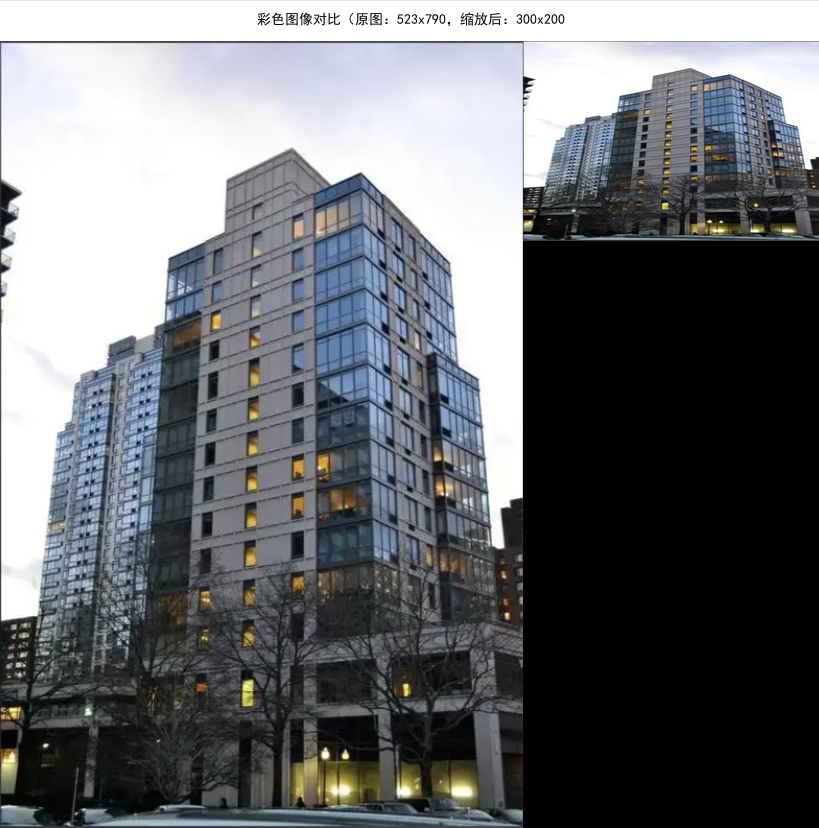
12.图像缩放

高质量图像缩放技术：插值与重采样

图像缩放是计算机视觉中预处理的核心操作（如统一输入尺寸、适配模型需求），代码通过 imresize 函数实现高质量缩放，核心技术是插值算法的选择。

缩放原理与插值方法

缩放本质：通过数学计算调整图像的像素数量，实现尺寸放大或缩小（代码中为缩小至 target_size）。
关键技术：使用 Image.LANCZOS 重采样算法（PIL 库中的高质量插值方法）：
- LANCZOS 插值基于 sinc 函数，通过计算周围多个像素的加权平均来生成新像素，尤其适合图像缩小场景。
- 优势：相比简单的双线性插值（BILINEAR）或最近邻插值（NEAREST），能更好地保留图像细节（如边缘、纹理），减少锯齿或模糊。
实现流程：
1. 将 NumPy 数组格式的图像转换为 PIL Image 对象（Image.fromarray）；
2. 调用 resize 方法，指定目标尺寸和插值算法（Image.LANCZOS）；
3. 转换回 NumPy 数组，便于后续处理。

跨平台中文字体适配：解决可视化标注乱码

在图像可视化中，中文标注乱码是常见问题，代码通过 find_chinese_font 函数实现系统字体的自动适配，确保标题和说明文字正常显示。

（1）字体查找策略

候选字体列表：按优先级排序常见中文字体（如 Windows 的 “SimHei”、macOS 的 “Heiti TC”、Linux 的 “WenQuanYi Micro Hei”），覆盖主流操作系统。
系统字体路径遍历：根据系统类型（Windows/macOS/ Linux）定向搜索字体目录（如 Windows 的 “C:/Windows/Fonts/”，Linux 的 “/usr/share/fonts/”），提高查找效率。
容错机制：若字体文件存在但加载失败（如权限问题），自动尝试下一个候选字体；若所有中文字体均不可用， fallback 到默认字体并提示警告。

（2）工程价值

确保对比图的标题（如 “彩色图像对比”）和尺寸信息（如 “原图：1024x768，缩放后：300x200”）清晰可读，避免因乱码影响结果理解。
增强代码的跨平台兼容性，在不同操作系统上保持一致的可视化效果。

对比图生成与可视化优化：直观展示缩放效果

create_comparison_image 函数负责将原图与缩放图拼接为对比图，并添加标题，核心目标是通过可视化直观呈现缩放前后的差异。

（1）图像拼接与布局设计

尺寸计算：总宽度为原图宽度与缩放图宽度之和，总高度为两者中的较大值，确保两张图像完整显示。
图像粘贴：通过 Image.paste 方法将原图粘贴在左侧、缩放图粘贴在右侧，形成横向对比布局，便于直观观察尺寸变化和细节保留情况。

（2）标题区域优化

独立标题区域：预留 40 像素高度的标题栏（背景为白色），与图像主体分离，避免遮挡图像内容。
文字居中算法：
1. 通过 draw.textbbox 计算标题文字的边界框，获取实际宽度；
2. 计算水平居中位置（(总宽度 - 文字宽度) // 2）和垂直居中位置，确保标题在视觉上居中对齐。
颜色适配：根据图像类型（彩色 / 灰度）调整文字颜色（灰度图用黑色文字，彩色图用黑色文字，与白色背景形成对比）。

彩色与灰度图像的差异化处理

代码同时支持彩色和灰度图像的缩放与对比，体现了计算机视觉中对不同图像类型的针对性处理思路。

（1）彩色图像处理

直接基于原始 RGB 三通道图像进行缩放，保留颜色信息；对比图采用 RGB 模式（mode=\'RGB\'），确保颜色不失真。

（2）灰度图像处理

先通过 img.convert(\'L\') 将彩色图像转换为单通道灰度图（像素值 0-255），再进行缩放；对比图采用灰度模式（mode=\'L\'），避免颜色干扰，聚焦亮度和细节变化。

（3）对比价值

通过横向对比（彩色原图 vs 彩色缩放图、灰度原图 vs 灰度缩放图），可直观观察：

缩放对颜色还原的影响（彩色图）；
缩放对边缘和纹理细节的保留能力（灰度图更易观察结构变化）。

Python代码如下：

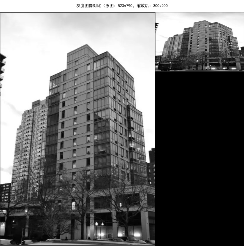
from PIL import Image, ImageDraw, ImageFontimport numpy as npimport osdef imresize(im, sz): \"\"\"使用PIL库调整图像大小（保持高质量）\"\"\" pil_im = Image.fromarray(np.uint8(im)) resized_pil = pil_im.resize(sz, Image.LANCZOS) # 高质量重采样 return np.array(resized_pil)def find_chinese_font(target_size=12): \"\"\"查找系统中可用的中文字体，确保中文正常显示\"\"\" # 常见中文字体列表（按优先级排序） font_candidates = [ \"SimHei.ttf\", # Windows 黑体 \"WenQuanYi Micro Hei.ttf\", # Linux 文泉驿微米黑 \"Heiti TC.ttc\", # macOS 黑体 \"Microsoft YaHei.ttc\", # Windows 微软雅黑 \"Arial Unicode.ttf\", # 跨平台通用字体 \"SimSun.ttc\" # Windows 宋体 ] # 系统字体路径（按系统类型匹配） system_font_paths = [] if os.name == \'nt\': # Windows系统 system_font_paths.append(\"C:/Windows/Fonts/\") elif os.name == \'posix\': # macOS/Linux系统 system_font_paths.extend([ \"/System/Library/Fonts/\", # macOS \"/Library/Fonts/\", # macOS \"/usr/share/fonts/truetype/\", # Linux \"/usr/share/fonts/opentype/\" # Linux ]) # 遍历路径查找可用字体 for path in system_font_paths: for font in font_candidates: full_path = os.path.join(path, font) if os.path.exists(full_path): try:  return ImageFont.truetype(full_path, target_size) except:  continue # 字体加载失败则尝试下一个 # 终极方案：使用默认字体（若所有中文字体加载失败） print(\"警告：未找到中文字体，使用默认字体（可能仍有乱码）\") return ImageFont.load_default()def create_comparison_image(original_img, resized_img, title=None, is_gray=False): \"\"\"创建原图与缩放图的对比图（优化字体显示）\"\"\" orig_width, orig_height = original_img.size resized_width, resized_height = resized_img.size # 计算对比图尺寸 total_width = orig_width + resized_width max_height = max(orig_height, resized_height) mode = \'L\' if is_gray else \'RGB\' # 创建对比图主体 comparison_img = Image.new(mode, (total_width, max_height)) comparison_img.paste(original_img, (0, 0)) comparison_img.paste(resized_img, (orig_width, 0)) # 添加标题（关键：使用支持中文的字体） if title: title_height = 40 # 标题区域高度 title_img = Image.new(mode, (total_width, title_height), color=255 if is_gray else (255, 255, 255)) draw = ImageDraw.Draw(title_img) # 加载中文字体（指定字号14） font = find_chinese_font(target_size=14) # 绘制标题（居中显示） if font: # 计算文字宽度，实现居中 text_bbox = draw.textbbox((0, 0), title, font=font) text_width = text_bbox[2] - text_bbox[0] text_x = (total_width - text_width) // 2 # 水平居中 text_y = (title_height - 20) // 2 # 垂直居中（20是字体大致高度） draw.text((text_x, text_y), title, font=font, fill=0 if is_gray else (0, 0, 0)) else: # fallback：无字体时默认绘制 draw.text((10, 10), title, fill=0 if is_gray else (0, 0, 0)) # 拼接标题和对比图 final_img = Image.new(mode, (total_width, max_height + title_height)) final_img.paste(title_img, (0, 0)) final_img.paste(comparison_img, (0, title_height)) return final_img return comparison_imgdef scale_and_save_image(input_path, output_color_path, output_gray_path, target_size): \"\"\"处理图像缩放并生成对比图（确保中文正常显示）\"\"\" try: with Image.open(input_path) as img: # 处理彩色图像 img_array = np.array(img) color_resized = Image.fromarray(imresize(img_array, target_size)) # 处理灰度图像 gray_img = img.convert(\'L\') gray_array = np.array(gray_img) gray_resized = Image.fromarray(imresize(gray_array, target_size)) # 生成彩色对比图（标题包含中文和尺寸信息） color_title = f\"彩色图像对比（原图：{img.size[0]}x{img.size[1]}，缩放后：{target_size[0]}x{target_size[1]}\" color_comparison = create_comparison_image(img, color_resized, color_title, is_gray=False) # 生成灰度对比图 gray_title = f\"灰度图像对比（原图：{img.size[0]}x{img.size[1]}，缩放后：{target_size[0]}x{target_size[1]}\" gray_comparison = create_comparison_image(gray_img, gray_resized, gray_title, is_gray=True) # 保存结果 color_comparison.save(output_color_path) gray_comparison.save(output_gray_path) print(f\"彩色对比图已保存至：{output_color_path}\") print(f\"灰度对比图已保存至：{output_gray_path}\") # 显示结果 color_comparison.show(title=\"彩色图像缩放对比\") gray_comparison.show(title=\"灰度图像缩放对比\") except FileNotFoundError: print(f\"错误：找不到文件 {input_path}\") except Exception as e: print(f\"处理错误：{e}\")if __name__ == \"__main__\": input_image = \"house2.jpg\" output_color = \"color_scaling_comparison.jpg\" output_gray = \"gray_scaling_comparison.jpg\" target_size = (300, 200) # 目标尺寸 scale_and_save_image(input_image, output_color, output_gray, target_size)

程序运行结果如下：

13.直方图均衡化

直方图均衡化的核心原理

直方图均衡化是一种对比度增强技术，其核心思想是通过数学变换将图像的像素值分布调整为更均匀的状态，从而扩展像素值的动态范围，使暗部更暗、亮部更亮，增强图像细节。

灰度图像均衡化（histeq函数）

实现步骤拆解：

计算原始直方图：通过 np.histogram 统计灰度图像中每个像素值（0-255）的出现频率，得到直方图 imhist。
计算累积分布函数（CDF）：对直方图进行累加求和（cumsum），得到 cdf，表示 “像素值小于等于某一阈值的概率”。
归一化 CDF：将 CDF 缩放到 0-255 范围（255 * cdf / cdf[-1]），确保映射后的像素值仍在有效区间。
像素值映射：通过 np.interp 将原始像素值根据 CDF 映射到新的像素值，实现均衡化。

效果：若原始图像直方图集中在某一区间（低对比度），均衡化后直方图会更平缓地分布在 0-255 范围，图像细节更清晰。

彩色图像均衡化（color_histeq函数）

彩色图像因包含 RGB 三通道，均衡化需考虑颜色一致性，代码采用分通道均衡化策略：

分离通道：将彩色图像拆分为红（R）、绿（G）、蓝（B）三个单通道。
独立均衡化：对每个通道分别应用灰度均衡化算法（调用 histeq）。
通道合并：将均衡化后的三通道重新组合为 RGB 图像。

特点：

优势：增强各颜色通道的对比度，使颜色更鲜艳、细节更突出。
局限：可能导致颜色失真（因三通道独立调整，破坏了原始颜色的比例关系），例如肤色可能偏色。实际应用中，更优方案是在 HSV 色彩空间均衡化亮度（V）通道，保持色调（H）和饱和度（S）不变。

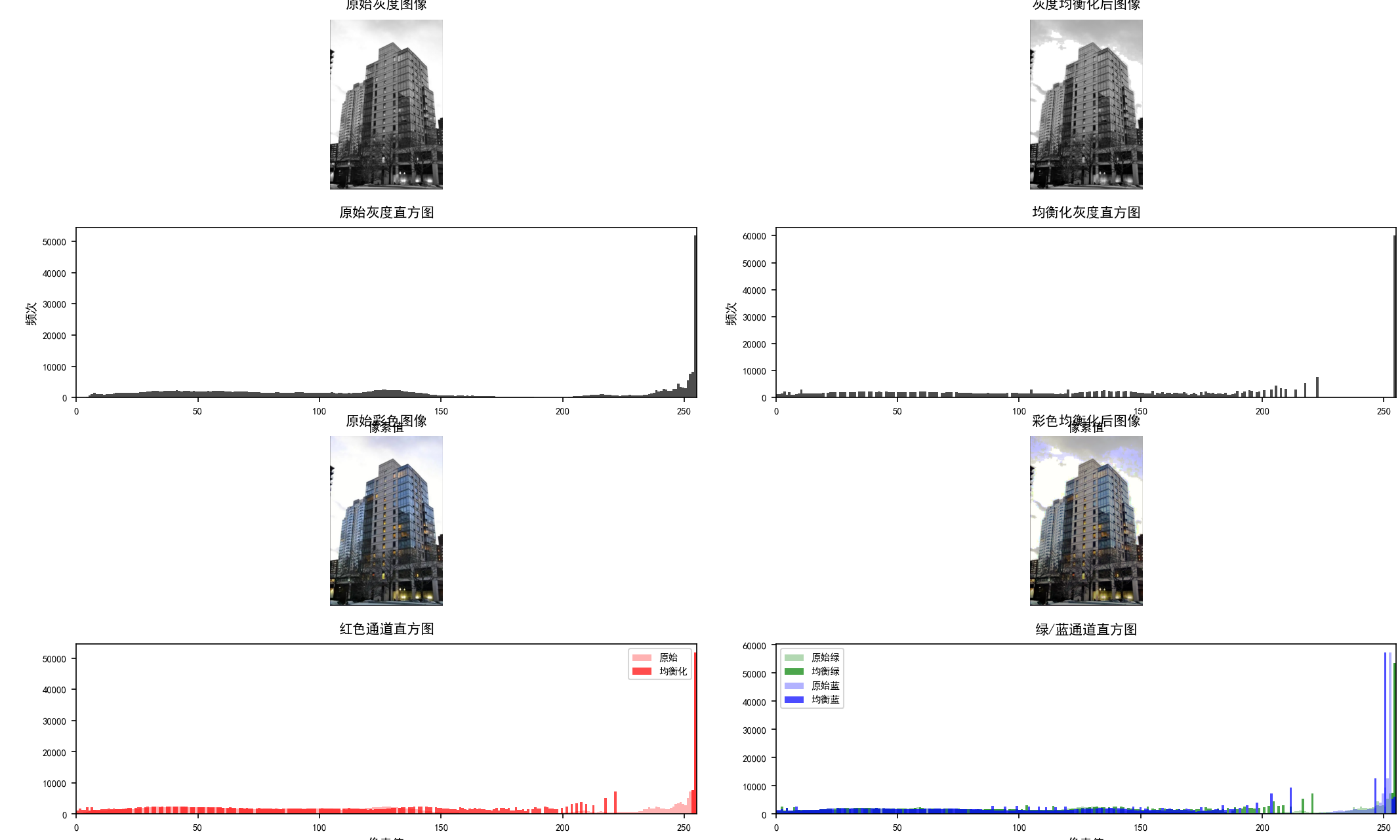
多维度可视化：对比均衡化效果

代码通过 4×2 的子图布局，系统展示均衡化前后的视觉效果和像素分布特征，形成完整的结果验证体系：

子图位置内容分析目标 (0,0) & (0,1) 原始灰度图 vs 均衡化灰度图直观对比灰度图像的视觉对比度变化 (1,0) & (1,1) 原始灰度直方图 vs 均衡化直方图量化像素值分布的变化（从集中到分散） (2,0) & (2,1) 原始彩色图 vs 均衡化彩色图展示彩色图像的整体视觉增强效果 (3,0) 红色通道原始 / 均衡化直方图单独分析红色分量的分布变化 (3,1) 绿 / 蓝通道原始 / 均衡化直方图对比绿、蓝分量的分布调整

可视化优化：

调整子图间距（hspace=0.4）和字体大小（刻度 7pt、标题 10pt），避免元素重叠；
直方图使用半透明效果（alpha=0.3/0.7）区分原始与均衡化结果，并用颜色对应通道（红 / 绿 / 蓝）；
限制 x 轴范围为 0-255（像素值范围），确保分布对比的准确性。

Python代码如下：

from PIL import Imageimport numpy as npimport matplotlib.pyplot as plt# 设置中文字体支持plt.rcParams[\"font.family\"] = [\"SimHei\"]plt.rcParams[\'axes.unicode_minus\'] = False # 解决负号显示问题plt.rcParams[\'axes.titlesize\'] = 10 # 减小标题字体plt.rcParams[\'axes.labelsize\'] = 9 # 减小标签字体plt.rcParams[\'legend.fontsize\'] = 8 # 减小图例字体def histeq(im, nbr_bins=256): \"\"\"单通道图像直方图均衡化\"\"\" imhist, bins = np.histogram(im.flatten(), nbr_bins, density=True) cdf = imhist.cumsum() cdf = 255 * cdf / cdf[-1] im2 = np.interp(im.flatten(), bins[:-1], cdf) return im2.reshape(im.shape), cdfdef color_histeq(rgb_image, nbr_bins=256): \"\"\"彩色图像分通道直方图均衡化\"\"\" r, g, b = rgb_image[:, :, 0], rgb_image[:, :, 1], rgb_image[:, :, 2] r_eq, _ = histeq(r, nbr_bins) g_eq, _ = histeq(g, nbr_bins) b_eq, _ = histeq(b, nbr_bins) return np.stack([r_eq, g_eq, b_eq], axis=2).astype(np.uint8)def visualize_histogram_equalization(input_path, output_path): \"\"\"优化布局的直方图均衡化可视化（解决字体重叠）\"\"\" try: # 读取图像 with Image.open(input_path) as img: rgb_orig = np.array(img) gray_orig = np.array(img.convert(\'L\')) # 执行均衡化 gray_eq, _ = histeq(gray_orig) color_eq = color_histeq(rgb_orig) # 创建4行2列布局（分散内容，避免拥挤） fig, axes = plt.subplots(4, 2, figsize=(12, 16)) # 增加高度到16，减少宽度到12 plt.subplots_adjust(hspace=0.4, wspace=0.2) # 增加垂直间距，减小水平间距 # -------------------- 灰度图像部分 -------------------- # 原始灰度图像 axes[0, 0].imshow(gray_orig, cmap=\'gray\') axes[0, 0].set_title(\'原始灰度图像\', pad=8) # 增加标题与图像间距 axes[0, 0].axis(\'off\') # 均衡化灰度图像 axes[0, 1].imshow(gray_eq, cmap=\'gray\') axes[0, 1].set_title(\'灰度均衡化后图像\', pad=8) axes[0, 1].axis(\'off\') # 原始灰度直方图 axes[1, 0].hist(gray_orig.flatten(), bins=256, color=\'black\', alpha=0.7) axes[1, 0].set_title(\'原始灰度直方图\', pad=8) axes[1, 0].set_xlabel(\'像素值\') axes[1, 0].set_ylabel(\'频次\') axes[1, 0].set_xlim([0, 255]) axes[1, 0].tick_params(axis=\'both\', labelsize=7) # 减小坐标轴刻度字体 # 均衡化灰度直方图 axes[1, 1].hist(gray_eq.flatten(), bins=256, color=\'black\', alpha=0.7) axes[1, 1].set_title(\'均衡化灰度直方图\', pad=8) axes[1, 1].set_xlabel(\'像素值\') axes[1, 1].set_ylabel(\'频次\') axes[1, 1].set_xlim([0, 255]) axes[1, 1].tick_params(axis=\'both\', labelsize=7) # -------------------- 彩色图像部分 -------------------- # 原始彩色图像 axes[2, 0].imshow(rgb_orig) axes[2, 0].set_title(\'原始彩色图像\', pad=8) axes[2, 0].axis(\'off\') # 均衡化彩色图像 axes[2, 1].imshow(color_eq) axes[2, 1].set_title(\'彩色均衡化后图像\', pad=8) axes[2, 1].axis(\'off\') # -------------------- 彩色通道直方图（分开展示，避免重叠） -------------------- # 红色通道对比 axes[3, 0].hist(rgb_orig[:, :, 0].flatten(), bins=256, color=\'red\', alpha=0.3, label=\'原始\') axes[3, 0].hist(color_eq[:, :, 0].flatten(), bins=256, color=\'red\', alpha=0.7, label=\'均衡化\') axes[3, 0].set_title(\'红色通道直方图\', pad=8) axes[3, 0].set_xlabel(\'像素值\') axes[3, 0].set_xlim([0, 255]) axes[3, 0].legend(fontsize=7) axes[3, 0].tick_params(axis=\'both\', labelsize=7) # 绿蓝通道合并对比（节省空间） axes[3, 1].hist(rgb_orig[:, :, 1].flatten(), bins=256, color=\'green\', alpha=0.3, label=\'原始绿\') axes[3, 1].hist(color_eq[:, :, 1].flatten(), bins=256, color=\'green\', alpha=0.7, label=\'均衡绿\') axes[3, 1].hist(rgb_orig[:, :, 2].flatten(), bins=256, color=\'blue\', alpha=0.3, label=\'原始蓝\') axes[3, 1].hist(color_eq[:, :, 2].flatten(), bins=256, color=\'blue\', alpha=0.7, label=\'均衡蓝\') axes[3, 1].set_title(\'绿/蓝通道直方图\', pad=8) axes[3, 1].set_xlabel(\'像素值\') axes[3, 1].set_xlim([0, 255]) axes[3, 1].legend(fontsize=7) axes[3, 1].tick_params(axis=\'both\', labelsize=7) # 调整布局并保存 plt.tight_layout() plt.savefig(output_path, dpi=300, bbox_inches=\'tight\') print(f\"结果已保存至: {output_path}\") plt.show() except FileNotFoundError: print(f\"错误：找不到图像文件 - {input_path}\") except Exception as e: print(f\"处理出错: {e}\")if __name__ == \"__main__\": input_image = \"house2.jpg\" output_image = \"fixed_histogram_equalization.jpg\" visualize_histogram_equalization(input_image, output_image)

程序运行结果如下：

14.图像平均

去雾算法的核心原理：大气散射模型

雾天图像的退化本质是光线在传播中被大气粒子散射，其物理模型可表示为：

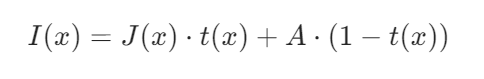
其中：

I(x)：雾天原图（输入图像）；
J(x)：去雾后的无雾图像（目标输出）；
t(x)：透射率（表示光线穿过雾后到达相机的比例，t=1 表示无雾，t→0 表示浓雾）；
A：大气光（雾的颜色，通常为灰白色）。

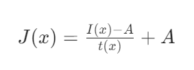
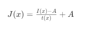
去雾的目标是从 I(x) 中估计 t(x) 和 A，再通过模型反推 J(x)：

核心步骤解析：从雾图到无雾图

代码通过四个关键步骤实现去雾，严格遵循暗通道先验算法的逻辑链：

（1）暗通道计算（darkchannel函数）：雾分布的直观反映

暗通道先验是算法的核心假设：在无雾图像中，除天空等特殊区域外，局部区域的最小像素值接近 0（即 “暗通道” 较暗）。而雾天图像的暗通道会因散射光而升高，因此暗通道图可间接反映雾的浓度（值越高，雾越浓）。

实现逻辑：
- 彩色图像：对每个像素的 RGB 三通道取最小值（np.min(img_array, axis=2)），得到单通道暗通道图；
- 灰度图像：直接使用灰度图作为暗通道（因单通道已反映亮度分布）。
作用：暗通道图是后续估计透射率和大气光的基础，其值高低与雾浓度正相关。

（2）大气光估计（airlight函数）：雾的颜色基准

大气光 A 是雾的主色调（通常为图像中最亮的区域，如天空、浓雾区域），准确估计 A 是去雾效果的关键。

实现逻辑：通过迭代区域分割与评分定位大气光：
不断将图像分割为 4 个区域，计算每个区域的 “亮度得分”（亮度均值 - 标准差，值越高表示区域越亮且均匀）；
选择得分最高的区域继续分割，直至区域足够小（像素数≤200）；
取该区域的最亮像素值作为大气光 A（彩色图取 RGB 值，灰度图取亮度值）。
优势：避免直接取全局最亮像素（可能是噪声或高光），通过区域迭代确保 A 代表真实雾色。

（3）透射率计算（transmission函数）：雾浓度的量化

透射率 t(x) 量化了雾的浓度，其值越低表示雾越浓。基于暗通道先验，透射率与暗通道值存在如下关系：

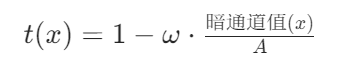
其中 ω 是修正系数（通常取 0.8-0.95），用于保留少量雾以避免过度去雾。

实现逻辑：
基于暗通道图和大气光 A，通过上述公式计算初始透射率；
限制透射率最小值为 tmin=0.1（避免分母过小导致图像失真）；
用3x3 加权均值滤波平滑透射率图（减少噪声，使雾浓度变化更连续）。
作用：透射率图直接决定去雾强度，平滑处理可避免去雾后图像出现块状 artifacts。

（4）去雾计算（defog函数）：无雾图像的重建

基于大气散射模型的反推公式，从原图、大气光和透射率计算去雾结果：

实现逻辑：
对彩色图像：将透射率图扩展为三通道（与原图通道匹配），确保每个颜色通道的去雾计算一致；
对灰度图像：直接单通道计算；
像素值裁剪：将结果限制在 0-255 范围（避免超出图像像素值有效区间）。
核心价值：通过物理模型反推，从雾图中还原无雾场景的细节（如边缘、纹理）。

彩色与灰度图像的差异化处理

代码同时支持彩色和灰度图像的去雾，针对不同通道特性优化流程：

图像类型暗通道计算大气光估计透射率处理去雾公式应用彩色 RGB 三通道取最小值取最亮区域的 RGB 值扩展为三通道透射率三通道分别计算后合并灰度直接使用灰度图取最亮区域的亮度值单通道透射率单通道直接计算

工程化优化：提升去雾效果与稳定性

代码在算法实现中加入多项工程优化，确保去雾效果更可靠：

（1）透射率最小值限制：通过 np.maximum(0.1, t) 避免透射率过低（t→0）导致的图像失真（分母过小会放大噪声）。

（2）透射率平滑：用 3x3 加权均值滤波（权重为 [1,2,1; 2,4,2; 1,2,1]）减少透射率图的噪声，使雾浓度变化更自然。

（3）大气光迭代估计：通过区域逐步分割定位最亮且均匀的区域，避免将高光或噪声误判为大气光。

Python代码如下：

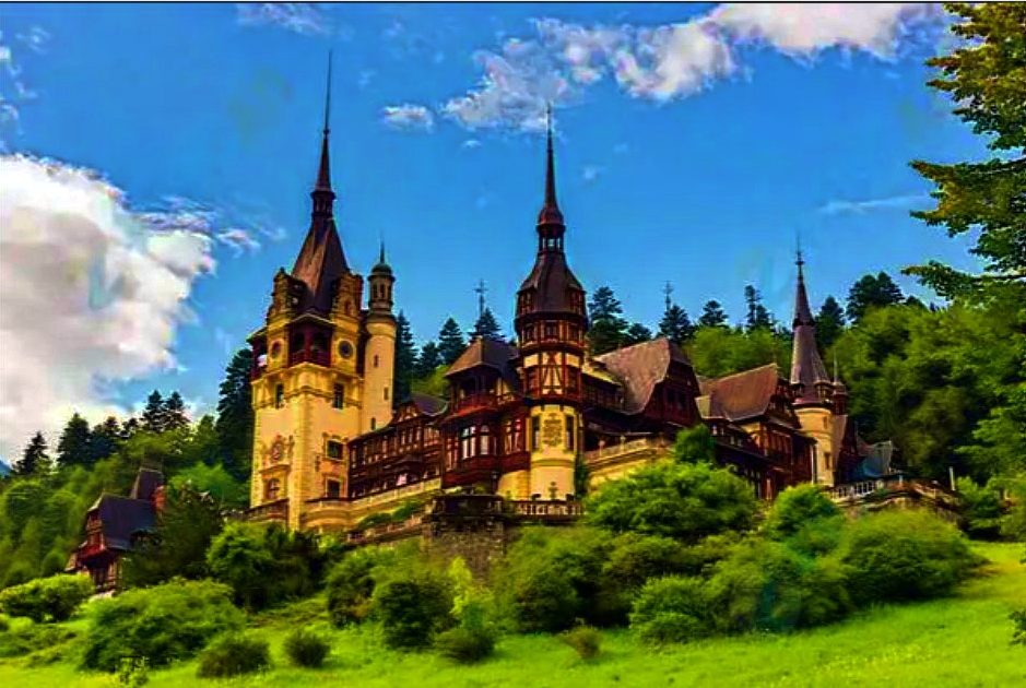
from PIL import Image, ImageStatimport numpy as npimport timedef darkchannel(input_img, is_gray=False): \"\"\"计算图像的暗通道（支持彩色和灰度）\"\"\" if is_gray: img_array = np.array(input_img).astype(np.float32) return Image.fromarray(img_array.astype(np.uint8)) else: img_array = np.array(input_img).astype(np.float32) dark = np.min(img_array, axis=2) # 计算每个像素的RGB最小值 return Image.fromarray(dark.astype(np.uint8))def airlight(input_img, is_gray=False): \"\"\"估计大气光值（支持彩色和灰度）\"\"\" img = input_img.copy() width, height = img.size max_iterations = 10 for _ in range(max_iterations): w_half = width // 2 h_half = height // 2 if w_half * h_half  max_intensity: max_intensity = intensity brightest_pixel = pixel return brightest_pixel # 将图像分为四个区域 regions = [ img.crop((0, 0, w_half, h_half)), # 左上 img.crop((w_half, 0, width, h_half)), # 右上 img.crop((0, h_half, w_half, height)), # 左下 img.crop((w_half, h_half, width, height)) # 右下 ] # 计算每个区域的得分 (亮度和-标准差) scores = [] for region in regions: stats = ImageStat.Stat(region) if is_gray: mean = stats.mean[0] stddev = stats.stddev[0] score = mean - stddev else: mean = stats.mean stddev = stats.stddev score = sum(mean) - sum(stddev) scores.append(score) # 选择得分最高的区域继续处理 max_idx = np.argmax(scores) img = regions[max_idx] width, height = img.size return 255 if is_gray else (255, 255, 255) # 默认返回白色def transmission(air, dark_img, omega=0.8, refine=True, is_gray=False): \"\"\"计算透射率图（支持彩色和灰度）\"\"\" dark_array = np.array(dark_img).astype(np.float32) if is_gray: A = air t = 1 - omega * dark_array / A else: A = max(air) t = 1 - omega * dark_array / A t = np.maximum(0.1, t) # 确保透射率不低于0.1 if refine: # 简单的均值滤波优化透射率图 t_smooth = np.copy(t) h, w = t.shape for i in range(1, h - 1): for j in range(1, w - 1): # 3x3加权平均 neighborhood = [  t[i - 1, j - 1], t[i - 1, j], t[i - 1, j + 1],  t[i, j - 1], t[i, j], t[i, j + 1],  t[i + 1, j - 1], t[i + 1, j], t[i + 1, j + 1] ] weights = [1, 2, 1, 2, 4, 2, 1, 2, 1] # 加权系数 t_smooth[i, j] = sum(n * w for n, w in zip(neighborhood, weights)) / 16 return t_smooth else: return tdef defog(img, t_map, air, t_min=0.1, is_gray=False): \"\"\"执行图像去雾（支持彩色和灰度）\"\"\" img_array = np.array(img).astype(np.float32) if is_gray: h, w = img_array.shape # 确保透射率不低于最小值 t_map = np.maximum(t_min, t_map) # 执行去雾计算 result = (img_array - air) / t_map + air # 裁剪像素值到0-255范围 result = np.clip(result, 0, 255).astype(np.uint8) return Image.fromarray(result) else: h, w, _ = img_array.shape # 确保透射率不低于最小值 t_map = np.maximum(t_min, t_map) # 扩展透射率图为三通道 t_expanded = np.expand_dims(t_map, axis=2) t_expanded = np.repeat(t_expanded, 3, axis=2) # 执行去雾计算 air_array = np.array(air).astype(np.float32) result = (img_array - air_array) / t_expanded + air_array # 裁剪像素值到0-255范围 result = np.clip(result, 0, 255).astype(np.uint8) return Image.fromarray(result)def main(): try: # 读取图像 img_path = \"castle1.jpg\" output_color_path = \"color_defogged_castle1.jpg\" output_gray_path = \"gray_defogged_castle1.jpg\" # 处理彩色图像 print(\"\\n===== 处理彩色图像 =====\") color_img = Image.open(img_path) width, height = color_img.size print(f\"图像尺寸: {width}x{height}\") # 彩色去雾参数 omega = 0.8 # 透射率调整参数 # 记录开始时间 start_time = time.time() print(\"计算暗通道...\") dark_image = darkchannel(color_img) print(\"估计大气光...\") air = airlight(color_img) print(f\"估计的大气光值: {air}\") print(\"计算透射率...\") t_map = transmission(air, dark_image, omega) print(\"执行去雾...\") color_fogfree_img = defog(color_img, t_map, air) # 记录结束时间 end_time = time.time() print(f\"彩色图像去雾完成，耗时: {end_time - start_time:.2f}秒\") # 保存彩色结果 color_fogfree_img.save(output_color_path) print(f\"彩色去雾后的图像已保存至: {output_color_path}\") # 处理灰度图像 print(\"\\n===== 处理灰度图像 =====\") gray_img = color_img.convert(\'L\') print(f\"图像尺寸: {width}x{height}\") # 记录开始时间 start_time = time.time() print(\"计算暗通道...\") gray_dark_image = darkchannel(gray_img, is_gray=True) print(\"估计大气光...\") gray_air = airlight(gray_img, is_gray=True) print(f\"估计的大气光值: {gray_air}\") print(\"计算透射率...\") gray_t_map = transmission(gray_air, gray_dark_image, omega, is_gray=True) print(\"执行去雾...\") gray_fogfree_img = defog(gray_img, gray_t_map, gray_air, is_gray=True) # 记录结束时间 end_time = time.time() print(f\"灰度图像去雾完成，耗时: {end_time - start_time:.2f}秒\") # 保存灰度结果 gray_fogfree_img.save(output_gray_path) print(f\"灰度去雾后的图像已保存至: {output_gray_path}\") # 显示结果 color_fogfree_img.show(title=\"彩色去雾结果\") gray_fogfree_img.show(title=\"灰度去雾结果\") except Exception as e: print(f\"处理过程中出错: {e}\")if __name__ == \"__main__\": main()

程序运行结果如下：

===== 处理彩色图像 =====
图像尺寸: 943x630
计算暗通道...
估计大气光...
估计的大气光值: (252, 251, 249)
计算透射率...
执行去雾...
彩色图像去雾完成，耗时: 8.06秒
彩色去雾后的图像已保存至: color_defogged_castle1.jpg

===== 处理灰度图像 =====
图像尺寸: 943x630
计算暗通道...
估计大气光...
估计的大气光值: 251
计算透射率...
执行去雾...
灰度图像去雾完成，耗时: 7.43秒
灰度去雾后的图像已保存至: gray_defogged_castle1.jpg

15.图像主成分分析

PCA 的核心原理：数据降维与特征保留

主成分分析（PCA）是一种经典的数据降维技术，其核心思想是通过线性变换将高维数据映射到低维空间，保留数据中最具代表性的特征（主成分），同时丢弃冗余信息。在图像处理中，PCA 可用于图像压缩、降噪或特征提取，用较少的主成分重建图像，平衡信息保留与数据量减少。

PCA 的数学实现（pca函数）

代码中pca函数实现了 PCA 的核心计算，步骤如下：

数据中心化：计算数据均值并减去均值，消除量纲影响（X = X - mean_X）；
协方差矩阵分析：根据数据维度与样本量的关系，选择不同的特征分解方法：
- 若维度高于样本量（dim > num_data），通过数据的协方差矩阵（X·Xᵀ）的特征值分解获取主成分；
- 若样本量高于维度，通过奇异值分解（SVD）直接获取主成分（U, S, V = np.linalg.svd(X)）；
主成分排序：按特征值（或奇异值）降序排列主成分，确保前 K 个主成分包含最多信息。

图像处理流程：从原图到 PCA 重建

代码对彩色和灰度图像分别执行 PCA 处理，核心流程为 “降采样→数据重塑→PCA 降维→图像重建→质量评估”，确保在减少计算量的同时有效展示 PCA 效果。

（1）降采样（Downsampling）

目的：通过DOWNSAMPLE_FACTOR（默认 8）降低图像分辨率（如 1024×768→128×96），减少像素数量，降低 PCA 计算复杂度。
实现：image.resize((width//factor, height//factor))，在保留图像整体结构的前提下减少数据量。

（2）图像数据重塑

PCA 要求输入为二维数据（样本数 × 特征数），因此需要将图像的二维像素矩阵重塑为高维向量：

灰度图像：单通道，形状为(rows, columns)，重塑为(rows×columns, 1)（每个像素作为一个样本，特征为亮度值）；
彩色图像：三通道，形状为(rows, columns, 3)，重塑为(rows×columns, 3)（每个像素作为一个样本，特征为 RGB 三通道值）。

（3）PCA 降维与图像重建

降维：选取前 K 个主成分（V_k = V[:K]），将中心化后的图像数据投影到主成分空间（projected = np.dot(X - mean_X, V_k.T)），得到低维表示；
重建：通过低维投影结果反推回原始空间（reconstructed = np.dot(projected, V_k) + mean_X），还原图像数据；
格式转换：将重建的二维数据重塑回图像尺寸（灰度图(rows, columns)，彩色图(rows, columns, 3)），并转换为uint8类型（像素值范围 0-255）。

质量评估：量化 PCA 重建效果

为客观衡量不同主成分数量（K）的重建质量，代码使用两种经典图像质量评估指标：

（1）峰值信噪比（PSNR）

定义：衡量重建图像与原图的像素值差异，公式为：

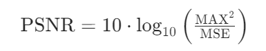
其中MAX为像素最大值（255），MSE为均方误差（像素值差异的平方均值）。
意义：值越高表示重建质量越好（失真越小），通常 PSNR > 30dB 时人眼难以察觉明显差异。

（2）结构相似性（SSIM）

定义：从亮度、对比度、结构三个维度衡量图像相似性，取值范围 0-1。
意义：值越接近 1 表示重建图像保留了更多原图的结构特征（如边缘、纹理），比 PSNR 更符合人眼视觉感知。

（3）评估逻辑

代码对不同 K 值的重建图像计算 PSNR 和 SSIM，结果显示：K 值越大，主成分保留的信息越多，PSNR 和 SSIM 越高，重建图像越接近原图；但 K 值增大也意味着降维效果减弱（数据量减少不明显）。

可视化对比：直观展示 PCA 效果

代码通过两种可视化方式对比 PCA 重建效果，清晰呈现主成分数量对图像质量的影响：

1. 单 K 值对比

将降采样原图与指定 K 值（默认 5）的重建图像横向拼接，添加标题标注图像尺寸、K 值及质量指标（PSNR/SSIM），直观展示单个 K 值的重建效果。

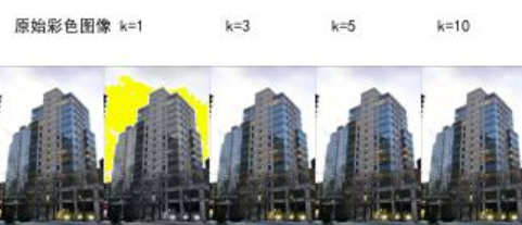
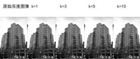
2. 多 K 值对比（K_VALUES = [1,3,5,10]）

将降采样原图与不同 K 值的重建图像横向拼接（从左到右：原图→K=1→K=3→K=5→K=10），通过对比可见：

K=1：仅保留最主要特征，图像模糊，细节丢失严重；
K=3：开始保留基本结构，但颜色 / 亮度仍有偏差；
K=5：大部分细节恢复，视觉上接近原图；
K=10：重建效果接近原图，几乎无明显失真。

彩色与灰度图像的差异化处理

代码针对两种图像类型优化 PCA 流程，适应不同通道特性：

图像类型数据维度主成分含义重建特点灰度图像单通道（1D 特征）亮度变化的主要模式重点保留明暗对比和边缘结构彩色图像三通道（3D 特征） RGB 颜色组合的主要模式同时保留亮度和颜色分布特征

工程化优化：提升可用性与可视化效果

代码包含多项工程优化，确保流程稳定且结果直观：

中文字体适配：find_font函数自动查找系统中文字体（如 SimHei、WenQuanYi），避免标题乱码；

字体大小自适应：calculate_font_size根据图像宽度和标题长度动态调整字体大小，确保标题完整显示；

鲁棒性处理：对小尺寸图像调整 SSIM 计算窗口（win_size），避免评估误差；处理字体加载失败等异常情况。

Python代码如下：

from PIL import Image, ImageDraw, ImageFontimport numpy as npfrom skimage.metrics import peak_signal_noise_ratio as psnrfrom skimage.metrics import structural_similarity as ssimimport os# -------------------- 参数配置区域 --------------------K = 5 # 主成分数量DOWNSAMPLE_FACTOR = 8 # 降采样因子INPUT_IMAGE = \'house2.jpg\' # 输入图像路径OUTPUT_COLOR_IMAGE = \'color_pca_comparison.jpg\' # 彩色对比图像路径OUTPUT_GRAY_IMAGE = \'gray_pca_comparison.jpg\' # 灰度对比图像路径MULTI_K_COLOR = \'multi_k_color.jpg\' # 彩色多k值对比MULTI_K_GRAY = \'multi_k_gray.jpg\' # 灰度多k值对比K_VALUES = [1, 3, 5, 10] # 多k值对比列表SHOW_IMAGES = True # 是否展示图像TITLE_FONT_SIZE = 20 # 标题字体大小TITLE_PADDING = 10 # 标题与图像的间距MAX_FONT_SIZE = 30 # 最大字体大小MIN_FONT_SIZE = 10 # 最小字体大小AUTO_FONT_SIZE = True # 是否根据图像宽度自动调整字体大小def pca(X): \"\"\"主成分分析：返回投影矩阵、方差和均值\"\"\" num_data, dim = X.shape mean_X = X.mean(axis=0) X = X - mean_X if dim > num_data: M = np.dot(X, X.T) e, EV = np.linalg.eigh(M) tmp = np.dot(X.T, EV).T V = tmp[::-1] S = np.sqrt(e)[::-1] for i in range(V.shape[1]): V[:, i] /= S else: U, S, V = np.linalg.svd(X) V = V[:num_data] return V, S, mean_Xdef find_font(target_size=20): \"\"\"查找系统可用的中文字体\"\"\" font_candidates = [ \"SimHei.ttf\", \"WenQuanYi Micro Hei.ttf\", \"Heiti TC.ttc\", \"SimSun.ttc\", \"Arial Unicode.ttf\" ] system_font_paths = [] if os.name == \'nt\': system_font_paths.append(\"C:/Windows/Fonts/\") elif os.name == \'posix\': system_font_paths.extend([ \"/System/Library/Fonts/\", \"/Library/Fonts/\", \"/usr/share/fonts/truetype/\", \"/usr/share/fonts/opentype/\" ]) for font_path_prefix in system_font_paths: for font in font_candidates: full_path = os.path.join(font_path_prefix, font) if os.path.exists(full_path): try:  return ImageFont.truetype(full_path, target_size) except Exception as e:  print(f\"无法加载字体 {full_path}: {e}\")  continue print(\"警告：未找到合适的中文字体，将使用默认字体\") try: return ImageFont.load_default() except: return Nonedef calculate_font_size(image_width, title_text): \"\"\"根据图像宽度自动计算字体大小\"\"\" if not AUTO_FONT_SIZE: return TITLE_FONT_SIZE base_size = min( MAX_FONT_SIZE, max(MIN_FONT_SIZE, int(image_width / (len(title_text) * 1.5))) ) return max(MIN_FONT_SIZE, min(MAX_FONT_SIZE, base_size))def add_title_to_image(image, title, font=None): \"\"\"在图像顶部添加标题\"\"\" if font is None: font_size = calculate_font_size(image.width, title) font = find_font(font_size) title_height = TITLE_FONT_SIZE + 2 * TITLE_PADDING new_height = image.height + title_height new_image = Image.new(\'RGB\', (image.width, new_height), color=(255, 255, 255)) new_image.paste(image, (0, title_height)) draw = ImageDraw.Draw(new_image) text_position = (TITLE_PADDING, TITLE_PADDING) if font: try: bbox = draw.textbbox((0, 0), title, font=font) text_width = bbox[2] - bbox[0] except AttributeError: text_width, _ = draw.textsize(title, font=font) if text_width > image.width - 2 * TITLE_PADDING: reduced_size = max(MIN_FONT_SIZE, int(font.size * 0.8)) print(f\"警告：标题文本太长，将字体从 {font.size} 调整为 {reduced_size}\") font = find_font(reduced_size) draw.text(text_position, title, font=font, fill=(0, 0, 0)) else: draw.text(text_position, title, fill=(0, 0, 0)) return new_imagedef add_titles_to_combined_image(image, titles, image_width, font=None): \"\"\"在拼接图像的每个子图上方添加标题\"\"\" if font is None: max_title_length = max(len(t) for t in titles) font_size = calculate_font_size(image_width, \"X\" * max_title_length) font = find_font(font_size) title_height = TITLE_FONT_SIZE + 2 * TITLE_PADDING new_height = image.height + title_height new_image = Image.new(\'RGB\', (image.width, new_height), color=(255, 255, 255)) new_image.paste(image, (0, title_height)) draw = ImageDraw.Draw(new_image) for i, title in enumerate(titles): text_position = (i * image_width + TITLE_PADDING, TITLE_PADDING) if font: try: bbox = draw.textbbox((0, 0), title, font=font) text_width = bbox[2] - bbox[0] except AttributeError: text_width, _ = draw.textsize(title, font=font) if text_width > image_width - 2 * TITLE_PADDING: reduced_size = max(MIN_FONT_SIZE, int(font.size * 0.8)) print(f\"警告：标题文本太长，将字体从 {font.size} 调整为 {reduced_size}\") reduced_font = find_font(reduced_size) draw.text(text_position, title, font=reduced_font, fill=(0, 0, 0)) else: draw.text(text_position, title, font=font, fill=(0, 0, 0)) else: draw.text(text_position, title, fill=(0, 0, 0)) return new_imagedef process_image(image, is_gray=False): \"\"\"处理单张图像（彩色或灰度）的PCA分析\"\"\" # 降采样 resized = image.resize((image.width // DOWNSAMPLE_FACTOR, image.height // DOWNSAMPLE_FACTOR)) print(f\"{\'灰度\' if is_gray else \'彩色\'}图像降采样后尺寸: {resized.size}\") # 转换为数组 if is_gray: # 灰度图为单通道 image_array = np.array(resized, dtype=np.float32) rows, columns = image_array.shape channels = 1 # 灰度图通道数为1 image_2d = image_array.reshape(rows * columns, channels) else: # 彩色图为三通道 image_array = np.array(resized, dtype=np.float32) rows, columns, channels = image_array.shape image_2d = image_array.reshape(rows * columns, channels) # PCA处理 print(f\"执行{\'灰度\' if is_gray else \'彩色\'}图像PCA计算，主成分数量: {K}\") V, S, mean_X = pca(image_2d) # 重建图像 V_k = V[:K] projected = np.dot(image_2d - mean_X, V_k.T) reconstructed = np.dot(projected, V_k) + mean_X # 恢复形状并转换为uint8 if is_gray: reconstructed_image_array = reconstructed.reshape(rows, columns) else: reconstructed_image_array = reconstructed.reshape(rows, columns, channels) reconstructed_image_array = np.uint8(reconstructed_image_array) reconstructed_image = Image.fromarray(reconstructed_image_array) # 质量评估 psnr_value = psnr(np.array(resized), reconstructed_image_array) min_size = min(resized.size) win_size = min_size if min_size % 2 == 1 else min_size - 1 win_size = max(3, win_size) if min_size < 3: print(\"警告：图像尺寸过小，SSIM计算可能不准确\") win_size = 1 try: if is_gray: # 灰度图SSIM计算（单通道） ssim_value = ssim(np.array(resized), reconstructed_image_array, data_range=255, win_size=win_size) else: # 彩色图SSIM计算（多通道） ssim_value = ssim(np.array(resized), reconstructed_image_array, multichannel=True, data_range=255, win_size=win_size, channel_axis=2) print(f\"{\'灰度\' if is_gray else \'彩色\'}图像质量评估:\") print(f\" PSNR: {psnr_value:.2f} dB\") print(f\" SSIM: {ssim_value:.4f}\") except Exception as e: print(f\"警告：无法计算{\'灰度\' if is_gray else \'彩色\'}图像SSIM: {e}\") ssim_value = None # 多k值对比图生成 width, height = resized.size combined_width = width * (len(K_VALUES) + 1) multi_combined = Image.new(\'RGB\', (combined_width, height)) multi_combined.paste(resized, (0, 0)) # 原始图像放最左 for i, k in enumerate(K_VALUES): print(f\" 处理{\'灰度\' if is_gray else \'彩色\'}图像k={k}的重建...\") V_k = V[:k] reconstructed_k = np.dot(np.dot(image_2d - mean_X, V_k.T), V_k) + mean_X if is_gray: reconstructed_k_array = reconstructed_k.reshape(rows, columns) else: reconstructed_k_array = reconstructed_k.reshape(rows, columns, channels) reconstructed_k_img = Image.fromarray(np.uint8(reconstructed_k_array)) multi_combined.paste(reconstructed_k_img, ((i + 1) * width, 0)) # 拼接原图与重建图（单k对比） combined = Image.new(\'RGB\', (width * 2, height)) combined.paste(resized, (0, 0)) combined.paste(reconstructed_image, (width, 0)) # 添加标题 titles = [f\"原始{\'灰度\' if is_gray else \'彩色\'}图像 ({width}x{height})\",  f\"PCA重建 (k={K})\"] if ssim_value is not None: titles[1] += f\", PSNR={psnr_value:.2f}dB, SSIM={ssim_value:.4f}\" font_size = calculate_font_size(width, max(titles, key=len)) font = find_font(font_size) titled_combined = add_titles_to_combined_image(combined, titles, width, font) # 多k值标题 multi_titles = [f\"原始{\'灰度\' if is_gray else \'彩色\'}图像\"] + [f\"k={k}\" for k in K_VALUES] multi_font_size = calculate_font_size(width, max(multi_titles, key=len)) multi_font = find_font(multi_font_size) titled_multi_combined = add_titles_to_combined_image(multi_combined, multi_titles, width, multi_font) return titled_combined, titled_multi_combined, resized.size# -------------------- 主流程 --------------------print(f\"正在处理图像: {INPUT_IMAGE}\")try: original_image = Image.open(INPUT_IMAGE) # 转换为灰度图 gray_image = original_image.convert(\'L\')except FileNotFoundError: print(f\"错误：找不到图像文件 \'{INPUT_IMAGE}\'\") exit(1)except Exception as e: print(f\"错误：打开图像失败: {e}\") exit(1)print(f\"原始彩色图像尺寸: {original_image.size}\")print(f\"原始灰度图像尺寸: {gray_image.size}\")# 处理彩色图像color_combined, color_multi, color_size = process_image(original_image, is_gray=False)# 处理灰度图像gray_combined, gray_multi, gray_size = process_image(gray_image, is_gray=True)# 保存结果try: color_combined.save(OUTPUT_COLOR_IMAGE) print(f\"彩色图像对比已保存至: {OUTPUT_COLOR_IMAGE}\") gray_combined.save(OUTPUT_GRAY_IMAGE) print(f\"灰度图像对比已保存至: {OUTPUT_GRAY_IMAGE}\") color_multi.save(MULTI_K_COLOR) print(f\"彩色多k值对比已保存至: {MULTI_K_COLOR}\") gray_multi.save(MULTI_K_GRAY) print(f\"灰度多k值对比已保存至: {MULTI_K_GRAY}\") if SHOW_IMAGES: print(\"显示彩色图像对比...\") color_combined.show(title=\"彩色图像 PCA 对比\") print(\"显示灰度图像对比...\") gray_combined.show(title=\"灰度图像 PCA 对比\") print(\"显示彩色多k值对比...\") color_multi.show(title=\"彩色图像 多k值 PCA 对比\") print(\"显示灰度多k值对比...\") gray_multi.show(title=\"灰度图像 多k值 PCA 对比\")except Exception as e: print(f\"错误：保存图像失败: {e}\")print(\"图像处理完成！\")

程序运行结果如下：

正在处理图像: house2.jpg
原始彩色图像尺寸: (523, 790)
原始灰度图像尺寸: (523, 790)
彩色图像降采样后尺寸: (65, 98)
执行彩色图像PCA计算，主成分数量: 5
彩色图像质量评估:
PSNR: 56.81 dB
SSIM: 1.0000
处理彩色图像k=1的重建...
处理彩色图像k=3的重建...
处理彩色图像k=5的重建...
处理彩色图像k=10的重建...
警告：标题文本太长，将字体从 10 调整为 10
警告：标题文本太长，将字体从 10 调整为 10
警告：标题文本太长，将字体从 10 调整为 10
灰度图像降采样后尺寸: (65, 98)
执行灰度图像PCA计算，主成分数量: 5
灰度图像质量评估:
PSNR: inf dB
SSIM: 1.0000
处理灰度图像k=1的重建...
处理灰度图像k=3的重建...
处理灰度图像k=5的重建...
处理灰度图像k=10的重建...
警告：标题文本太长，将字体从 10 调整为 10
警告：标题文本太长，将字体从 10 调整为 10
警告：标题文本太长，将字体从 10 调整为 10
彩色图像对比已保存至: color_pca_comparison.jpg
灰度图像对比已保存至: gray_pca_comparison.jpg
彩色多k值对比已保存至: multi_k_color.jpg
灰度多k值对比已保存至: multi_k_gray.jpg
显示彩色图像对比...
显示灰度图像对比...
显示彩色多k值对比...
显示灰度多k值对比...
图像处理完成！

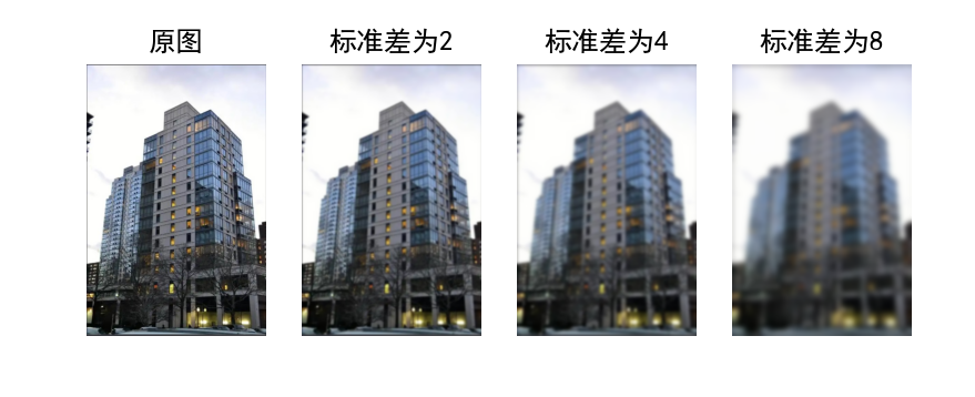
16.图像模糊

高斯模糊的核心原理

高斯模糊是一种基于高斯函数的线性平滑滤波技术，通过对图像中每个像素及其邻域像素进行加权平均，实现图像模糊效果。其核心原理是：距离中心像素越近的像素权重越高，距离越远权重越低，权重分布符合二维高斯函数：

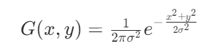
其中，σ（标准差）是控制模糊程度的关键参数：

σ 越小：高斯核（权重窗口）越集中，模糊效果越弱，保留更多细节；
σ 越大：高斯核越分散，模糊效果越强，图像细节丢失越多。

灰度图像的高斯模糊处理

代码首先对灰度图像（单通道）应用高斯模糊，流程如下：

图像加载与转换：

通过 Image.open(\'house2.jpg\').convert(\'L\') 将彩色图像转换为灰度图像（单通道，像素值 0-255）；
用 array() 转换为 NumPy 数组，便于数值计算。

高斯滤波实现：

使用 scipy.ndimage.filters.gaussian_filter(im, blur) 应用高斯模糊，其中 blur 即 σ（代码中测试了 2、4、8 三个值）；
滤波后通过 np.uint8(im2) 将结果转回 8 位整数类型（确保像素值在 0-255 范围）。

效果对比：

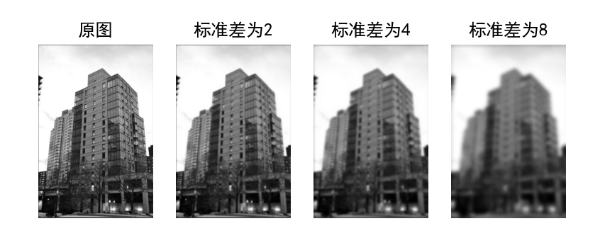
子图布局为 1×4，从左到右依次展示：原图→σ=2→σ=4→σ=8；
随着 σ 增大，图像边缘逐渐模糊，纹理细节（如墙面纹理、窗户轮廓）逐渐消失，整体变得更平滑。

彩色图像的高斯模糊处理

彩色图像（RGB 三通道）的模糊处理需考虑通道独立性，代码采用分通道模糊策略：

图像加载：

直接加载彩色图像为 NumPy 数组（形状为 (高度, 宽度, 3)），保留 RGB 三通道。

分通道高斯滤波：

对 R、G、B 三个通道分别应用高斯滤波（for i in range(3): im2[:, :, i] = filters.gaussian_filter(im[:, :, i], blur)）；

确保每个颜色通道的模糊程度一致，避免色彩偏移。

效果对比：

布局与灰度图一致，展示原图及不同 σ 的模糊效果；
彩色模糊不仅平滑亮度细节，也模糊颜色过渡边界（如物体边缘的颜色变化），但因三通道同步处理，不会破坏原图的色彩平衡。

可视化设计与结果分析

代码通过 Matplotlib 构建对比图，清晰呈现模糊效果的变化规律：

布局设计：

灰度图和彩色图分别使用 1×4 子图布局，左侧为原图，右侧依次为不同 σ 的结果；
关闭坐标轴（axis(\'off\')）并添加标题（title(u\'标准差为\' + imNum)），聚焦图像本身的视觉变化。

关键结论：

σ=2：轻微模糊，去除高频噪声（如细小纹理），保留主要结构；
σ=4：中等模糊，边缘开始平滑，细节明显减少；
σ=8：强模糊，图像整体趋于平滑，仅保留大尺度区域（如房屋轮廓、天空）。

Python代码如下：

from PIL import Imagefrom numpy import *from pylab import *from scipy.ndimage import filtersfrom matplotlib.font_manager import FontPropertiesplt.rcParams[\'font.sans-serif\'] = [\'SimHei\'] # 显示中文标签im = array(Image.open(\'house2.jpg\').convert(\'L\'))figure()gray()axis(\'off\')subplot(141)axis(\'off\')title(u\'原图\')imshow(im)for bi, blur in enumerate([2, 4, 8]): im2 = zeros(im.shape) im2 = filters.gaussian_filter(im, blur) im2 = np.uint8(im2) imNum = str(blur) subplot(1, 4, 2 + bi) axis(\'off\') title(u\'标准差为\' + imNum) imshow(im2)savefig(\'gray_image_blur_house2.jpg\')show()im = array(Image.open(\'house2.jpg\'))figure()axis(\'off\')subplot(141)axis(\'off\')title(u\'原图\')imshow(im)for bi, blur in enumerate([2, 4, 8]): im2 = zeros(im.shape) for i in range(3): im2[:, :, i] = filters.gaussian_filter(im[:, :, i], blur) im2 = np.uint8(im2) imNum = str(blur) subplot(1, 4, 2 + bi) axis(\'off\') title(u\'标准差为\' + imNum) imshow(im2)savefig(\'color_image_blur_house2.jpg\')show()

程序运行结果如下：

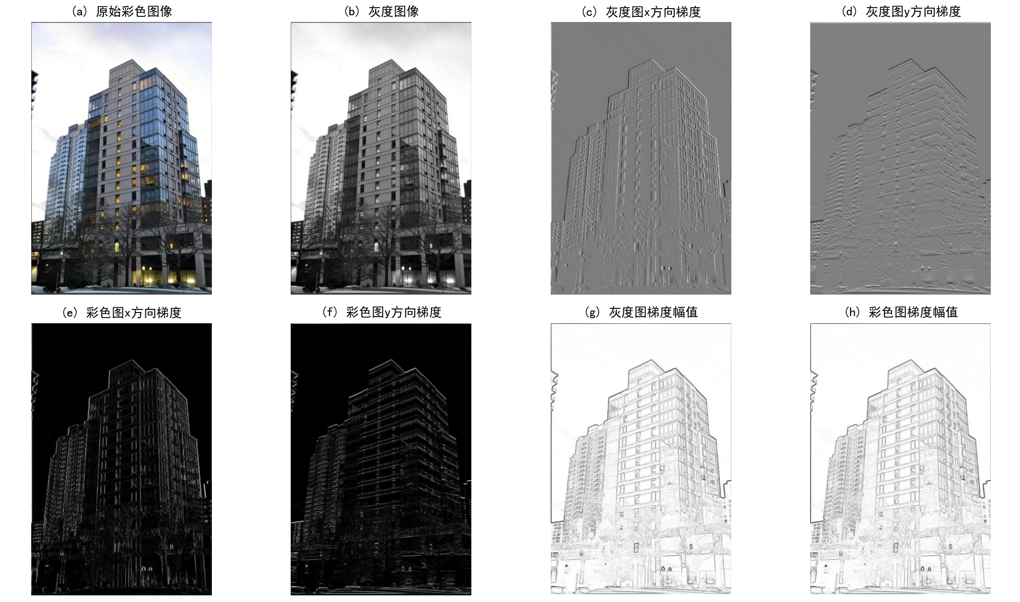
17.图像导数

边缘检测的核心原理：梯度与 Sobel 算子

边缘是图像中像素值快速变化的区域（如物体轮廓、纹理边界），其本质是像素灰度 / 颜色的突变。Sobel 边缘检测通过计算图像的梯度（变化率）来定位边缘，核心原理是：

梯度是向量，包含方向（变化最快的方向）和幅值（变化强度）；
边缘区域的梯度幅值较大，可通过阈值筛选定位边缘。

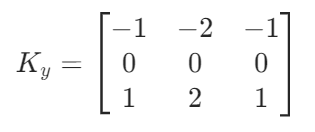
Sobel 算子通过两个 3×3 卷积核（分别对应 x 方向和 y 方向）与图像卷积，近似计算梯度：

x 方向核（检测垂直边缘）：
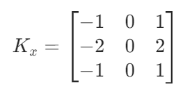
y 方向核（检测水平边缘）：

灰度图像的 Sobel 边缘检测

灰度图像（单通道）的边缘检测流程直观，代码通过以下步骤实现：

梯度计算：

用filters.sobel(gray_image, axis=1, output=gray_dx)计算 x 方向梯度（垂直边缘响应）；
用filters.sobel(gray_image, axis=0, output=gray_dy)计算 y 方向梯度（水平边缘响应）。

梯度幅值：

通过公式 gray_mag = np.sqrt(gray_dx² + gray_dy²) 计算梯度强度，幅值越大表示边缘越明显。

归一化：

将梯度值映射到 0-255 范围（(mag - min)/(max - min) * 255），确保可视化效果清晰。

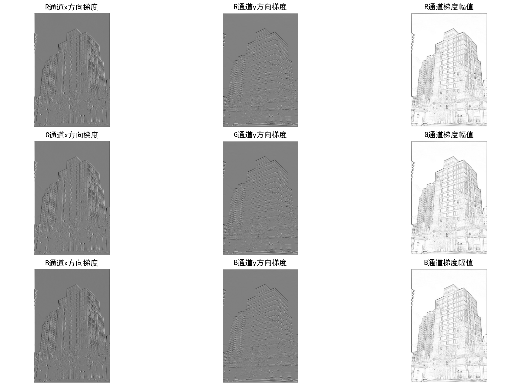
彩色图像的 Sobel 边缘检测：分通道策略

彩色图像（RGB 三通道）的边缘不仅取决于亮度变化，还与颜色变化相关。代码采用分通道梯度融合策略，保留各颜色通道的边缘特征：

分通道梯度计算（channel_sobel函数）

对 R、G、B 三个通道分别执行 Sobel 检测：

每个通道独立计算 x 方向梯度（dx）、y 方向梯度（dy）和梯度幅值（mag = sqrt(dx² + dy²)）；
例如，红色通道（R）的梯度反映红色分量的变化边缘（如红色物体的轮廓），绿色通道（G）反映绿色分量的变化边缘。

整体梯度融合

将三通道的梯度信息融合为彩色图像的整体梯度：

整体 x 方向梯度：overall_dx = sqrt(rx² + gx² + bx²)（融合三通道的垂直边缘响应）；
整体 y 方向梯度：overall_dy = sqrt(ry² + gy² + by²)（融合三通道的水平边缘响应）；
整体梯度幅值：overall_mag = sqrt(overall_dx² + overall_dy²)（综合所有通道的边缘强度）。

优势

分通道处理避免了直接将彩色图转灰度后检测的信息丢失（例如，彩色图中颜色差异明显但亮度差异小的边缘，在灰度图中可能被忽略，而分通道融合可保留这类边缘）。

可视化设计：多维度梯度特征对比

代码通过精心设计的可视化布局，直观展示边缘检测的关键特征，分为两个核心对比图：

灰度与彩色边缘对比图（2×4 布局）

子图位置内容核心意义 (a) 原始彩色图像提供边缘检测的原始参考 (b) 灰度图像展示亮度信息的简化版本 (c) 灰度图 x 方向梯度突出垂直边缘（如房屋的竖直线条） (d) 灰度图 y 方向梯度突出水平边缘（如屋顶的水平线） (e) 彩色图 x 方向梯度融合颜色通道的垂直边缘，更丰富 (f) 彩色图 y 方向梯度融合颜色通道的水平边缘，更丰富 (g) 灰度图梯度幅值（反色）灰度视角的所有边缘汇总 (h) 彩色图梯度幅值（反色）彩色视角的所有边缘汇总，细节更多

彩色通道边缘对比图（3×3 布局）

按 R、G、B 通道分别展示梯度特征：

每个通道的 x 方向梯度图：展示该颜色分量的垂直边缘；
每个通道的 y 方向梯度图：展示该颜色分量的水平边缘；
每个通道的梯度幅值图（反色）：汇总该通道的所有边缘。

示例：红色通道的梯度幅值图可能突出红色物体的边缘（如红色屋顶），蓝色通道可能突出天空与建筑的边界。

Python代码如下：

from PIL import Imageimport numpy as npimport matplotlib.pyplot as pltfrom scipy.ndimage import filters# 设置中文显示plt.rcParams[\"font.family\"] = [\"SimHei\"]plt.rcParams[\'axes.unicode_minus\'] = False # 解决负号显示问题def sobel_edge_detection(rgb_image): \"\"\"对彩色图像执行Sobel边缘检测\"\"\" # 分离RGB三个通道 r, g, b = rgb_image[:, :, 0], rgb_image[:, :, 1], rgb_image[:, :, 2] # 为每个通道计算x和y方向的梯度 def channel_sobel(channel): dx = np.zeros_like(channel, dtype=np.float32) dy = np.zeros_like(channel, dtype=np.float32) filters.sobel(channel, axis=1, output=dx) # x方向 filters.sobel(channel, axis=0, output=dy) # y方向 mag = np.sqrt(dx ** 2 + dy ** 2) # 梯度幅值 return dx, dy, mag # 计算各通道梯度 rx, ry, r_mag = channel_sobel(r) gx, gy, g_mag = channel_sobel(g) bx, by, b_mag = channel_sobel(b) # 计算彩色图像的整体梯度（各通道梯度的平方和开方） overall_dx = np.sqrt(rx ** 2 + gx ** 2 + bx ** 2) overall_dy = np.sqrt(ry ** 2 + gy ** 2 + by ** 2) overall_mag = np.sqrt(overall_dx ** 2 + overall_dy ** 2) # 归一化处理 def normalize(arr): return (arr - arr.min()) / (arr.max() - arr.min() + 1e-8) * 255 # 归一化所有梯度 rx, ry, r_mag = map(normalize, [rx, ry, r_mag]) gx, gy, g_mag = map(normalize, [gx, gy, g_mag]) bx, by, b_mag = map(normalize, [bx, by, b_mag]) overall_dx, overall_dy, overall_mag = map(normalize, [overall_dx, overall_dy, overall_mag]) return { \'channels\': { \'R\': (rx, ry, r_mag), \'G\': (gx, gy, g_mag), \'B\': (bx, by, b_mag) }, \'overall\': (overall_dx, overall_dy, overall_mag) }# 读取图像（保留彩色信息）try: # 同时读取彩色图和灰度图 color_image = np.array(Image.open(\'house2.jpg\'), dtype=np.float32) gray_image = np.array(Image.open(\'house2.jpg\').convert(\'L\'), dtype=np.float32)except FileNotFoundError: print(\"错误：未找到图像文件 \'house2.jpg\'\") exit(1)# 执行彩色图像边缘检测color_edges = sobel_edge_detection(color_image)# 执行灰度图像边缘检测（用于对比）gray_dx = np.zeros_like(gray_image)gray_dy = np.zeros_like(gray_image)filters.sobel(gray_image, axis=1, output=gray_dx)filters.sobel(gray_image, axis=0, output=gray_dy)gray_mag = np.sqrt(gray_dx ** 2 + gray_dy ** 2)gray_mag = (gray_mag - gray_mag.min()) / (gray_mag.max() - gray_mag.min() + 1e-8) * 255# 创建显示窗口（2行4列布局）plt.figure(figsize=(16, 8))# 1. 原始图像plt.subplot(241)plt.imshow(np.uint8(color_image))plt.title(\'(a) 原始彩色图像\')plt.axis(\'off\')plt.subplot(242)plt.imshow(gray_image, cmap=\'gray\')plt.title(\'(b) 灰度图像\')plt.axis(\'off\')# 2. 灰度图边缘检测结果plt.subplot(243)plt.imshow(gray_dx, cmap=\'gray\')plt.title(\'(c) 灰度图x方向梯度\')plt.axis(\'off\')plt.subplot(244)plt.imshow(gray_dy, cmap=\'gray\')plt.title(\'(d) 灰度图y方向梯度\')plt.axis(\'off\')# 3. 彩色图整体梯度plt.subplot(245)plt.imshow(color_edges[\'overall\'][0], cmap=\'gray\')plt.title(\'(e) 彩色图x方向梯度\')plt.axis(\'off\')plt.subplot(246)plt.imshow(color_edges[\'overall\'][1], cmap=\'gray\')plt.title(\'(f) 彩色图y方向梯度\')plt.axis(\'off\')# 4. 梯度幅值对比plt.subplot(247)plt.imshow(255 - gray_mag, cmap=\'gray\') # 反色显示plt.title(\'(g) 灰度图梯度幅值\')plt.axis(\'off\')plt.subplot(248)plt.imshow(255 - color_edges[\'overall\'][2], cmap=\'gray\') # 反色显示plt.title(\'(h) 彩色图梯度幅值\')plt.axis(\'off\')# 调整布局并保存plt.tight_layout()plt.savefig(\'color_image_derivative_house2.jpg\', dpi=300, bbox_inches=\'tight\')plt.show()# 额外显示各颜色通道的边缘检测结果plt.figure(figsize=(15, 10))channels = [\'R\', \'G\', \'B\']for i, channel in enumerate(channels): dx, dy, mag = color_edges[\'channels\'][channel] plt.subplot(331 + i * 3) plt.imshow(dx, cmap=\'gray\') plt.title(f\'{channel}通道x方向梯度\') plt.axis(\'off\') plt.subplot(332 + i * 3) plt.imshow(dy, cmap=\'gray\') plt.title(f\'{channel}通道y方向梯度\') plt.axis(\'off\') plt.subplot(333 + i * 3) plt.imshow(255 - mag, cmap=\'gray\') # 反色显示 plt.title(f\'{channel}通道梯度幅值\') plt.axis(\'off\')plt.tight_layout()plt.savefig(\'color_channels_derivative_house2.jpg\', dpi=300, bbox_inches=\'tight\')plt.show()

程序运行结果如下：

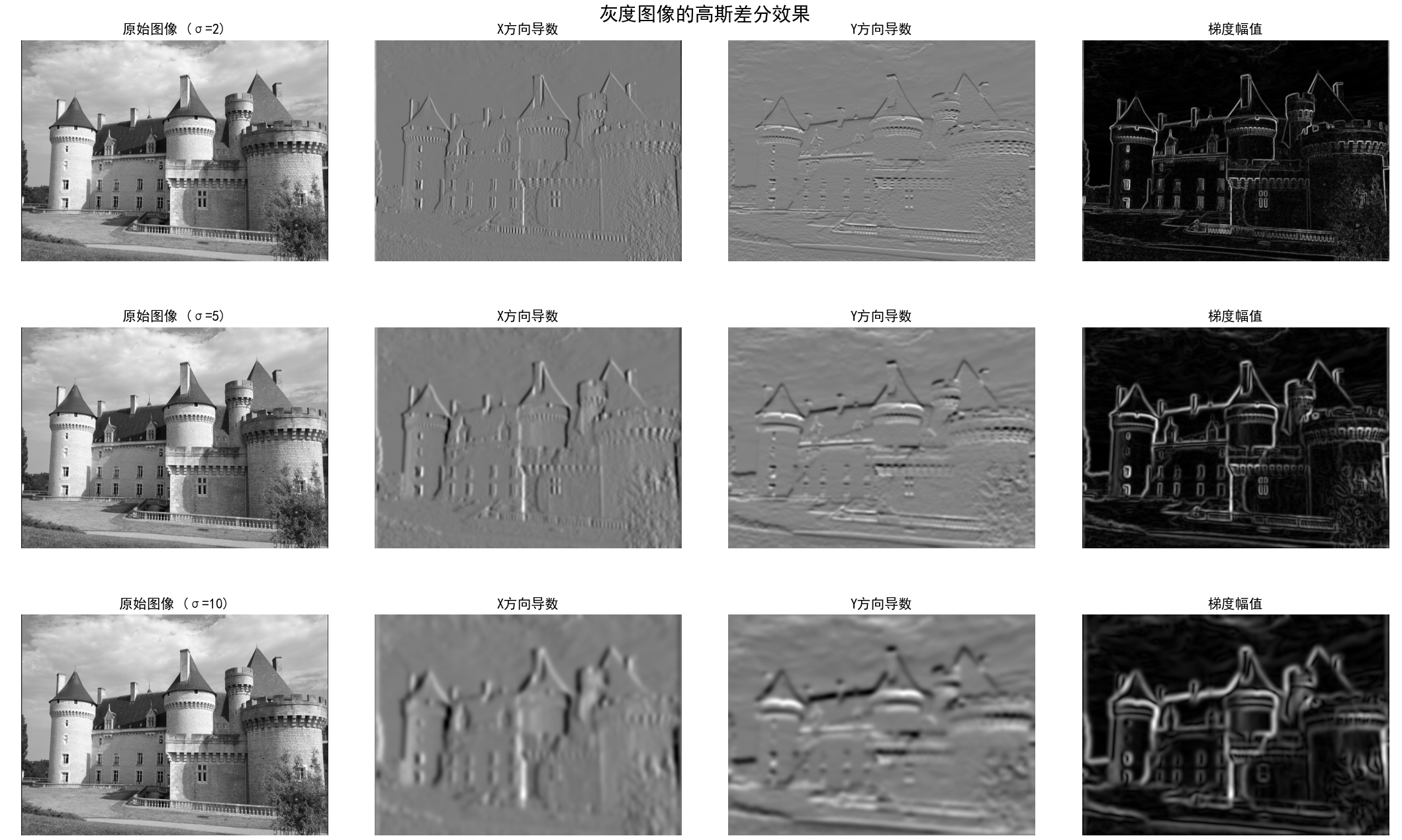
18.图像高斯差分操作

核心原理：高斯导数与多尺度分析

高斯导数是平滑与求导的结合技术，其核心思想是：先通过高斯滤波对图像进行平滑（减少噪声），再计算平滑后图像的导数（捕捉像素变化率）。通过调整高斯核的标准差σ，可实现不同尺度的特征提取：

σ 越小：高斯核越窄，平滑效果弱，导数对细节（如细小纹理、噪声）更敏感，捕捉小尺度边缘；
σ 越大：高斯核越宽，平滑效果强，导数对大尺度结构（如物体轮廓）更敏感，过滤细节噪声。

高斯导数的数学基础是：对图像 I 先进行高斯卷积 Gσ，再求偏导：

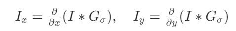
其中 ∗ 表示卷积，Ix 和 Iy 分别为 x 方向（垂直变化）和 y 方向（水平变化）的导数，梯度幅值为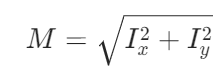（反映边缘强度）。

灰度图像的高斯导数计算（compute_derivatives函数）

该函数实现灰度图像的多尺度梯度提取，核心步骤如下：

高斯导数计算

使用 scipy.ndimage.filters.gaussian_filter 同时完成平滑与求导：
- filters.gaussian_filter(im, sigma, (0, 1), imgx)：计算 x 方向导数（垂直边缘响应），参数 (0,1) 表示对第二维度（宽度方向）求导；
- filters.gaussian_filter(im, sigma, (1, 0), imgy)：计算 y 方向导数（水平边缘响应），参数 (1,0) 表示对第一维度（高度方向）求导。

梯度优化与归一化

绝对值修正：对导数取绝对值（imgx_abs = np.abs(imgx)），确保梯度强度仅反映变化幅度（忽略正负方向，便于可视化）；
幅值计算：通过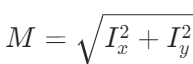计算梯度幅值，综合 x 和 y 方向的变化强度；
归一化：将梯度幅值映射到 0-255 范围（(mag - min)/(max - min) * 255），避免因数值范围过小导致可视化失真。

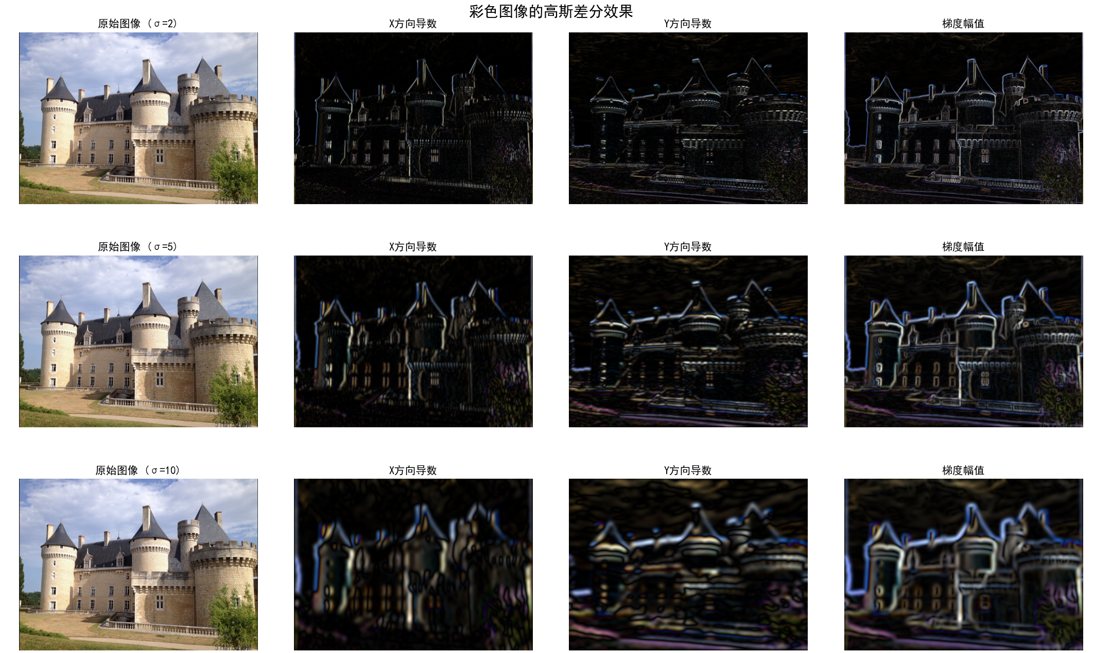
彩色图像的高斯导数计算（process_color_image函数）

彩色图像（RGB 三通道）的梯度提取需保留各颜色通道的独立特征，代码采用分通道处理策略：

通道分离：将彩色图像拆分为 R、G、B 三通道（r, g, b = color_img[:, :, 0], ...）；

单通道梯度计算：对每个通道分别调用 compute_derivatives，得到各通道的 x 导数、y 导数和梯度幅值；

通道融合：将三通道的导数结果重新组合为彩色梯度图（color_x = np.stack([r_x, g_x, b_x], axis=2)），保留颜色通道的梯度特性。

优势：彩色图像的边缘不仅依赖亮度变化，还依赖颜色变化（如红色与绿色的边界）。分通道处理可捕捉不同颜色分量的边缘，避免直接转灰度后丢失颜色相关的边缘信息。

多尺度可视化：不同 σ 下的梯度特征对比

代码通过 visualize_results 函数构建多尺度对比图，直观展示不同σ（代码中为 2、5、10）对梯度特征的影响，布局设计如下：

灰度图像可视化（1 列 ×3 行，每行对应一个 σ）

子图位置内容核心观察每行第 1 列原始灰度图像提供梯度计算的参考基准每行第 2 列 x 方向导数（垂直边缘） σ=2：细节丰富（如墙面纹理）；σ=10：仅保留大轮廓（如城堡边缘）每行第 3 列 y 方向导数（水平边缘） σ=2：小尺度水平纹理清晰；σ=10：仅保留大尺度水平结构（如屋顶线）每行第 4 列梯度幅值（边缘强度） σ 增大，边缘逐渐平滑，细节噪声减少，大尺度边缘更突出

彩色图像可视化（结构同灰度图）

原始彩色图像保留颜色信息，作为参考；
x/y 方向导数通过绝对值归一化处理（color_x_vis = (np.abs(color_x) / max) * 255），确保彩色通道的导数差异可可视化；
梯度幅值图融合三通道的边缘强度，颜色对应原始通道的梯度贡献（如红色通道梯度强的区域在幅值图中偏红）。

Python代码如下：

from PIL import Imageimport numpy as npimport matplotlib.pyplot as pltfrom scipy.ndimage import filters# 设置中文显示plt.rcParams[\"font.family\"] = [\"SimHei\"]plt.rcParams[\'axes.unicode_minus\'] = False # 解决负号显示问题plt.rcParams[\'axes.titlesize\'] = 10 # 减小标题字体大小def compute_derivatives(im, sigma): \"\"\"计算图像在指定sigma下的x导数、y导数和梯度幅值（修正版本）\"\"\" imgx = np.zeros_like(im, dtype=np.float32) imgy = np.zeros_like(im, dtype=np.float32) # 计算高斯导数（x和y方向） filters.gaussian_filter(im, sigma, (0, 1), imgx) # x方向导数 filters.gaussian_filter(im, sigma, (1, 0), imgy) # y方向导数 # 关键修正1：对导数取绝对值，确保梯度强度反映变化幅度 imgx_abs = np.abs(imgx) imgy_abs = np.abs(imgy) # 计算梯度幅值（基于绝对值的平方和） imgmag = np.sqrt(imgx_abs ** 2 + imgy_abs ** 2) # 关键修正2：优化归一化，避免数值范围过小导致的放大问题 mag_max = imgmag.max() mag_min = imgmag.min() if mag_max - mag_min < 1e-8: # 若梯度几乎无变化，直接置为0 imgmag = np.zeros_like(imgmag) else: imgmag = (imgmag - mag_min) / (mag_max - mag_min) * 255 # 归一化到0-255 return imgx, imgy, imgmagdef process_color_image(color_img, sigma): \"\"\"处理彩色图像，分别计算RGB三个通道的导数\"\"\" r, g, b = color_img[:, :, 0], color_img[:, :, 1], color_img[:, :, 2] r_x, r_y, r_mag = compute_derivatives(r, sigma) g_x, g_y, g_mag = compute_derivatives(g, sigma) b_x, b_y, b_mag = compute_derivatives(b, sigma) color_x = np.stack([r_x, g_x, b_x], axis=2) color_y = np.stack([r_y, g_y, b_y], axis=2) color_mag = np.stack([r_mag, g_mag, b_mag], axis=2) return color_x, color_y, color_magdef visualize_results(gray_img, color_img, sigmas): \"\"\"可视化不同sigma值下的结果\"\"\" fig_height = 5 * len(sigmas) fig_width = 14 # 灰度图像结果 plt.figure(figsize=(fig_width, fig_height)) plt.suptitle(\'灰度图像的高斯差分效果\', fontsize=14, y=0.99) for i, sigma in enumerate(sigmas): imgx, imgy, imgmag = compute_derivatives(gray_img, sigma) plt.subplot(len(sigmas), 4, i * 4 + 1) plt.imshow(gray_img, cmap=\'gray\') plt.title(f\'原始图像 (σ={sigma})\', pad=5) plt.axis(\'off\') plt.subplot(len(sigmas), 4, i * 4 + 2) plt.imshow(imgx, cmap=\'gray\') plt.title(f\'X方向导数\', pad=5) plt.axis(\'off\') plt.subplot(len(sigmas), 4, i * 4 + 3) plt.imshow(imgy, cmap=\'gray\') plt.title(f\'Y方向导数\', pad=5) plt.axis(\'off\') plt.subplot(len(sigmas), 4, i * 4 + 4) plt.imshow(imgmag, cmap=\'gray\') plt.title(f\'梯度幅值\', pad=5) plt.axis(\'off\') plt.tight_layout(rect=[0, 0, 1, 0.98]) plt.subplots_adjust(hspace=0.3) plt.savefig(\'gray_gaussian_difference.jpg\', dpi=300, bbox_inches=\'tight\') # 彩色图像结果 plt.figure(figsize=(fig_width, fig_height)) plt.suptitle(\'彩色图像的高斯差分效果\', fontsize=14, y=0.99) for i, sigma in enumerate(sigmas): color_x, color_y, color_mag = process_color_image(color_img, sigma) plt.subplot(len(sigmas), 4, i * 4 + 1) plt.imshow(color_img.astype(np.uint8)) plt.title(f\'原始图像 (σ={sigma})\', pad=5) plt.axis(\'off\') # 对导数取绝对值并归一化（解决彩色导数全黑问题） color_x_vis = np.abs(color_x) color_x_vis = (color_x_vis / (color_x_vis.max() + 1e-8)) * 255 plt.subplot(len(sigmas), 4, i * 4 + 2) plt.imshow(color_x_vis.astype(np.uint8)) plt.title(f\'X方向导数\', pad=5) plt.axis(\'off\') color_y_vis = np.abs(color_y) color_y_vis = (color_y_vis / (color_y_vis.max() + 1e-8)) * 255 plt.subplot(len(sigmas), 4, i * 4 + 3) plt.imshow(color_y_vis.astype(np.uint8)) plt.title(f\'Y方向导数\', pad=5) plt.axis(\'off\') plt.subplot(len(sigmas), 4, i * 4 + 4) plt.imshow(color_mag.astype(np.uint8)) plt.title(f\'梯度幅值\', pad=5) plt.axis(\'off\') plt.tight_layout(rect=[0, 0, 1, 0.98]) plt.subplots_adjust(hspace=0.3) plt.savefig(\'color_gaussian_difference.jpg\', dpi=300, bbox_inches=\'tight\') plt.show()# 主程序if __name__ == \"__main__\": try: # 读取图像 gray_img = np.array(Image.open(\'castle3.jpg\').convert(\'L\'), dtype=np.float32) color_img = np.array(Image.open(\'castle3.jpg\'), dtype=np.float32) except FileNotFoundError: print(\"错误：未找到图像文件 \'castle3.jpg\'\") exit(1) except Exception as e: print(f\"图像读取错误: {e}\") exit(1) sigmas = [2, 5, 10] # 不同的高斯核标准差 visualize_results(gray_img, color_img, sigmas)

程序运行结果如下：

19.图像的形态学

核心技术框架：二值化与形态学分析的完整流程

代码的核心逻辑是通过 “像素阈值分割→连通区域标记→形态学噪声去除” 的三阶流程，实现图像中目标区域的提取与优化。该流程是目标检测、图像分割等任务的基础预处理步骤，核心目标是从复杂图像中分离出感兴趣的目标区域（前景）与背景。

第一步：图像二值化（Binary Thresholding）

二值化是将灰度 / 彩色图像转换为仅含黑白两种像素的图像（像素值非 0 即 1），通过阈值筛选突出目标区域。代码针对彩色和灰度图像设计了差异化但对称的二值化策略：

彩色图像的二值化

直接二值化：基于 RGB 三通道的联合阈值（(R < r_threshold) & (G < g_threshold) & (B < b_threshold)），仅保留三通道值均低于阈值的像素（视为目标）。这种方式适合目标在 RGB 三通道均具有低亮度特征的场景（如深色物体）。
转灰度后二值化：先将彩色图像转为灰度图（convert(\'L\')），再用单一灰度阈值（128）分割（im_gray_from_color < 128）。这种方式将彩色信息简化为亮度信息，适合目标与背景的亮度差异显著的场景。

灰度图像的二值化

直接二值化：用单一灰度阈值（128）分割（im_gray < gray_threshold），将亮度低于阈值的像素视为目标。
形式对称处理：为保持与彩色流程的对称性，设计 “灰度→灰度后二值化”（逻辑与直接二值化一致），确保对比的公平性。

二值化的核心价值：通过阈值筛选去除冗余信息，将复杂图像简化为 “目标 - 背景” 的二元结构，为后续区域分析奠定基础。

第二步：连通区域标记（Connected Component Labeling）

二值化后图像中可能包含多个独立的目标区域，代码通过连通区域标记技术识别并计数这些区域，实现目标的初步量化。

技术实现

通过 scipy.ndimage.measurements.label 函数实现：

原理：遍历二值化图像，将相邻的前景像素（值为 1）归为同一区域，用唯一整数标记（如区域 1、区域 2…）；
输出：标记后的图像（每个区域用不同数值表示）和区域数量（nbr_color、nbr_gray等）。

分析价值

区域数量反映二值化结果的 “纯净度”：数量过多可能意味着噪声干扰（如小斑点被误判为目标）；
标记图像直观展示目标的空间分布（如区域大小、位置），为后续筛选重要目标提供依据。

第三步：形态学优化（Morphological Opening）

二值化和标记后通常存在噪声（如小斑点、区域边缘毛刺），代码通过形态学开运算去除噪声，优化区域形态。

开运算原理

开运算是 “腐蚀（Erosion）→膨胀（Dilation）” 的组合操作：

腐蚀：收缩目标区域边界，去除小噪声和细毛刺；
膨胀：扩张目标区域边界，恢复腐蚀导致的有效区域收缩。
代码中使用 5×5 的结构元素（structuring_element = np.ones((5,5))）和 2 次迭代，平衡噪声去除与区域保留。

效果

通过 morphology.binary_opening 处理后：

小噪声区域（如孤立的前景像素）被去除；
区域边界更平滑，连通性更合理；
区域数量减少（对比开运算前后的 nbr_open 与原始 nbr），体现噪声被过滤。

对称化可视化：彩色与灰度处理的对比分析

代码设计 3×4 的子图布局，严格对称展示彩色和灰度图像的处理全流程，直观对比差异：

行 / 列彩色图像处理（左 2 列）灰度图像处理（右 2 列）核心对比点第 1 行原始彩色图→彩色直接二值化原始灰度图→灰度直接二值化二值化方式对区域提取的影响第 2 行彩色→灰度二值化→彩色二值化标记灰度→灰度二值化→灰度二值化标记区域数量与分布的初始差异第 3 行彩色转灰度开运算标记→彩色直接开运算标记灰度转灰度开运算标记→灰度直接开运算标记形态学操作对不同图像类型的优化效果

关键结论：彩色与灰度处理的差异分析

通过区域数量对比和可视化结果，可得出以下规律：

二值化方式影响：彩色直接二值化（基于 RGB 联合阈值）可能比 “彩色→灰度二值化” 保留更多颜色相关的目标细节（如特定颜色的小区域）；

噪声敏感度：彩色图像因多通道信息，二值化后可能引入更多噪声区域（区域数量更多），而灰度图像因信息简化，初始噪声较少；

形态学效果：开运算对两种图像类型均能有效去除小噪声，且灰度图像的优化效果更稳定（区域数量减少更显著）。

Python代码如下：

from PIL import Imageimport numpy as npimport matplotlib.pyplot as pltfrom scipy.ndimage import measurements, morphology# 设置中文字体plt.rcParams[\"font.family\"] = [\"SimHei\"]plt.rcParams[\'axes.unicode_minus\'] = False # 解决负号显示问题def image_binary_analysis(image_path): \"\"\" 同时处理彩色图像和灰度图像，保持完全相同的处理流程和展示形式 \"\"\" try: # 读取原始彩色图像 with Image.open(image_path) as img: im_color = np.array(img) # 彩色图像数组 (H, W, 3) im_gray = np.array(img.convert(\'L\')) # 转换为灰度图像 (H, W) # -------------------- 彩色图像处理流程 -------------------- # 1. 彩色直接二值化（基于RGB阈值） r_threshold, g_threshold, b_threshold = 100, 100, 100 binary_color_direct = ( (im_color[:, :, 0] < r_threshold) & (im_color[:, :, 1] < g_threshold) & (im_color[:, :, 2] < b_threshold) ) # 2. 彩色图像的灰度二值化（作为对比） im_gray_from_color = np.array(Image.fromarray(im_color).convert(\'L\')) binary_gray_from_color = (im_gray_from_color < 128) # 3. 形态学处理（开运算+标记） structuring_element = np.ones((5, 5)) # 彩色直接二值化后续处理 labels_color, nbr_color = measurements.label(binary_color_direct) im_open_color = morphology.binary_opening(binary_color_direct, structuring_element, iterations=2) labels_open_color, nbr_open_color = measurements.label(im_open_color) # 彩色转灰度后二值化的后续处理 labels_gray_color, nbr_gray_color = measurements.label(binary_gray_from_color) im_open_gray_color = morphology.binary_opening(binary_gray_from_color, structuring_element, iterations=2) labels_open_gray_color, nbr_open_gray_color = measurements.label(im_open_gray_color) # -------------------- 灰度图像处理流程（与彩色保持完全一致） -------------------- # 1. 灰度直接二值化（对应彩色直接二值化） gray_threshold = 128 # 灰度阈值（对应彩色的三通道阈值逻辑） binary_gray_direct = (im_gray < gray_threshold) # 2. 灰度图像的\"灰度二值化\"（形式上对应，实际与直接二值化逻辑一致） binary_gray_from_gray = (im_gray < gray_threshold) # 与直接二值化相同，保持结构对称 # 3. 形态学处理（与彩色使用完全相同的参数） # 灰度直接二值化后续处理 labels_gray, nbr_gray = measurements.label(binary_gray_direct) im_open_gray = morphology.binary_opening(binary_gray_direct, structuring_element, iterations=2) labels_open_gray, nbr_open_gray = measurements.label(im_open_gray) # 灰度转灰度后二值化的后续处理（形式上对应） labels_gray_gray, nbr_gray_gray = measurements.label(binary_gray_from_gray) im_open_gray_gray = morphology.binary_opening(binary_gray_from_gray, structuring_element, iterations=2) labels_open_gray_gray, nbr_open_gray_gray = measurements.label(im_open_gray_gray) # -------------------- 可视化对比（保持完全相同的布局结构） -------------------- # 3行4列布局：左侧4列彩色处理，右侧4列灰度处理 fig, axes = plt.subplots(3, 4, figsize=(20, 15)) plt.subplots_adjust(hspace=0.4, wspace=0.1) # -------------------- 第一行：原始图像与直接二值化 -------------------- # 彩色原始图像 axes[0, 0].imshow(im_color) axes[0, 0].set_title(\'1. 彩色原始图像\') axes[0, 0].axis(\'off\') # 彩色直接二值化 axes[0, 1].imshow(binary_color_direct, cmap=\'gray\') axes[0, 1].set_title(f\'2. 彩色直接二值化（R<{r_threshold}, G<{g_threshold}, B<{b_threshold}）\') axes[0, 1].axis(\'off\') # 灰度原始图像 axes[0, 2].imshow(im_gray, cmap=\'gray\') axes[0, 2].set_title(\'1. 灰度原始图像\') axes[0, 2].axis(\'off\') # 灰度直接二值化 axes[0, 3].imshow(binary_gray_direct, cmap=\'gray\') axes[0, 3].set_title(f\'2. 灰度直接二值化（阈值 <{gray_threshold}）\') axes[0, 3].axis(\'off\') # -------------------- 第二行：灰度转换后二值化与标记结果 -------------------- # 彩色转灰度后二值化 axes[1, 0].imshow(binary_gray_from_color, cmap=\'gray\') axes[1, 0].set_title(\'3. 彩色→灰度后二值化（阈值128）\') axes[1, 0].axis(\'off\') # 彩色二值化标记结果 axes[1, 1].imshow(labels_color, cmap=\'viridis\') axes[1, 1].set_title(f\'4. 彩色二值化标记（{nbr_color}个区域）\') axes[1, 1].axis(\'off\') # 灰度→灰度后二值化（形式对应） axes[1, 2].imshow(binary_gray_from_gray, cmap=\'gray\') axes[1, 2].set_title(f\'3. 灰度→灰度后二值化（阈值 <{gray_threshold}）\') axes[1, 2].axis(\'off\') # 灰度二值化标记结果 axes[1, 3].imshow(labels_gray, cmap=\'viridis\') axes[1, 3].set_title(f\'4. 灰度二值化标记（{nbr_gray}个区域）\') axes[1, 3].axis(\'off\') # -------------------- 第三行：开运算后标记结果 -------------------- # 彩色开运算后标记 axes[2, 0].imshow(labels_open_gray_color, cmap=\'viridis\') axes[2, 0].set_title(f\'5. 彩色→灰度开运算后（{nbr_open_gray_color}个区域）\') axes[2, 0].axis(\'off\') # 彩色直接二值化开运算后标记 axes[2, 1].imshow(labels_open_color, cmap=\'viridis\') axes[2, 1].set_title(f\'6. 彩色直接二值化开运算后（{nbr_open_color}个区域）\') axes[2, 1].axis(\'off\') # 灰度→灰度开运算后标记 axes[2, 2].imshow(labels_open_gray_gray, cmap=\'viridis\') axes[2, 2].set_title(f\'5. 灰度→灰度开运算后（{nbr_open_gray_gray}个区域）\') axes[2, 2].axis(\'off\') # 灰度直接二值化开运算后标记 axes[2, 3].imshow(labels_open_gray, cmap=\'viridis\') axes[2, 3].set_title(f\'6. 灰度直接二值化开运算后（{nbr_open_gray}个区域）\') axes[2, 3].axis(\'off\') # 总标题与保存 plt.suptitle(\'彩色图像 vs 灰度图像 二值化处理全流程对比\', fontsize=16) plt.tight_layout(rect=[0, 0, 1, 0.97]) output_path = \'color_vs_gray_binary_analysis.jpg\' plt.savefig(output_path, dpi=300) print(f\"结果已保存为: {output_path}\") plt.show() # 数量对比表格 print(\"\\n【区域数量对比表】\") print(f\"彩色图像处理:\") print(f\" 直接二值化: {nbr_color} → 开运算后: {nbr_open_color}\") print(f\" 转灰度后二值化: {nbr_gray_color} → 开运算后: {nbr_open_gray_color}\") print(f\"\\n灰度图像处理:\") print(f\" 直接二值化: {nbr_gray} → 开运算后: {nbr_open_gray}\") print(f\" 转灰度后二值化: {nbr_gray_gray} → 开运算后: {nbr_open_gray_gray}\") except FileNotFoundError: print(f\"错误：未找到图像文件 \'{image_path}\'\") except Exception as e: print(f\"处理出错：{e}\")if __name__ == \"__main__\": image_binary_analysis(\"castle3.jpg\")

程序运行结果如下：

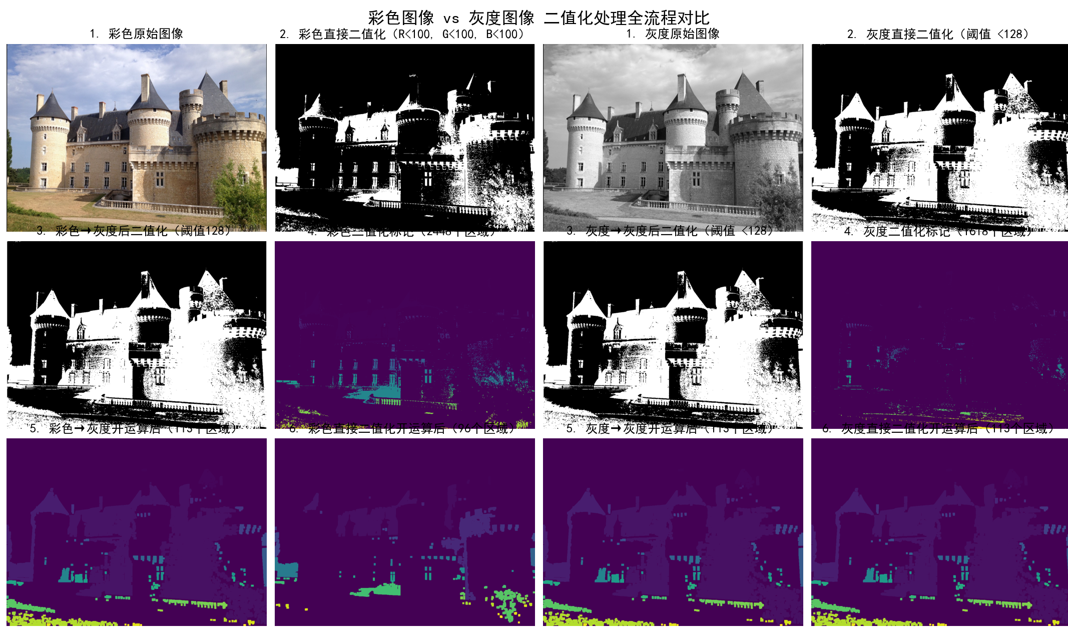
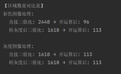
20.图像降噪

高斯噪声图像降噪原理

高斯噪声的特性

高斯噪声（Gaussian Noise）是一种加性噪声，其像素值的偏差服从高斯分布（正态分布）。数学上，若原始图像像素值为 f(x,y)，噪声图像像素值为 g(x,y)，则：

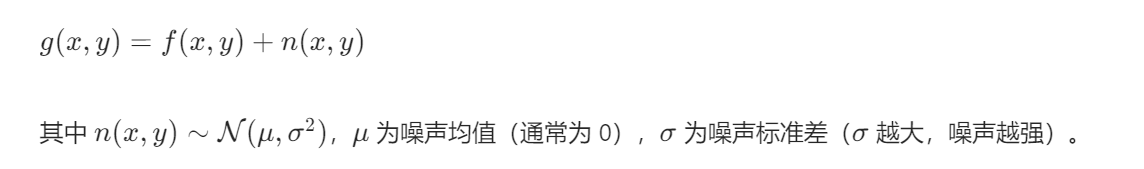
高斯噪声的视觉表现为图像整体呈现 “颗粒感”，噪声均匀分布在整个图像中，没有明显的局部聚集，每个像素都可能受到轻微干扰（如低光照下的传感器噪声）。

高斯噪声的降噪核心思路

高斯噪声的降噪核心是平滑滤波：通过对像素及其邻域进行加权平均，削弱高频噪声的波动，同时尽量保留图像的低频结构（如边缘、纹理）。由于噪声服从高斯分布，邻域内的正常像素值通常集中在均值附近，而噪声的随机波动会被平均抵消。

典型降噪方法及原理

高斯滤波（Gaussian Filtering）

原理：使用高斯核（权重符合高斯分布的卷积核）与图像卷积，对每个像素的邻域进行加权平均。高斯核的权重随距离中心像素的距离增大而减小，公式为：

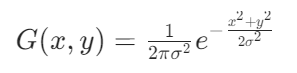
其中 (x,y) 为核内像素相对中心的坐标，σ 为高斯核的标准差（控制平滑程度）。
优势：平滑效果均匀，能有效抑制高斯噪声，且不会过度模糊边缘（相比均值滤波）。
应用：适用于轻微至中度高斯噪声，是预处理的常用方法。

均值滤波（Mean Filtering）

原理：使用固定大小的矩形核（如 3×3、5×5），将每个像素替换为邻域内所有像素的平均值：

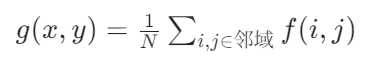
其中 N 为邻域像素数量。
优势：计算简单，对轻度高斯噪声有效。
局限：过度平滑会模糊边缘和细节，适合对细节要求不高的场景。

双边滤波（Bilateral Filtering）

原理：在高斯滤波基础上增加像素值相似度权重，同时考虑空间距离和像素值差异：
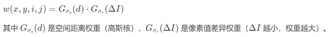
优势：在平滑噪声的同时保留边缘（边缘处像素值差异大，权重低，避免过度模糊）。
应用：适用于需要保边的高斯噪声图像（如人像、风景）。

高斯模糊与差分（高斯金字塔降噪）

原理：对图像进行多尺度高斯模糊，通过不同尺度的差异提取噪声（噪声在高频尺度更明显），再从原图中减去噪声估计。
优势：适应不同强度的高斯噪声，保留更多细节。

椒盐噪声图像降噪原理

椒盐噪声的特性

椒盐噪声（Salt-and-Pepper Noise）是一种脉冲噪声，表现为图像中随机出现的极端值像素：“盐噪声”（Salt Noise）为纯白像素（值为 255），“椒噪声”（Pepper Noise）为纯黑像素（值为 0）。其数学模型为：

椒盐噪声的视觉表现为图像中散布的黑白斑点，噪声像素与周围正常像素的差异极大，但受影响的像素比例通常较低（如传输错误、传感器故障导致）。

椒盐噪声的降噪核心思路

椒盐噪声的降噪核心是噪声检测与替换：由于噪声像素是极端值（0或255），与正常像素差异显著，因此先识别噪声像素，再用邻域内的正常像素值替换噪声像素，避免噪声扩散。

典型降噪方法及原理

中值滤波（Median Filtering）

原理：使用固定大小的滑动窗口（如3×3），将窗口内所有像素值排序后取中值，替换窗口中心的像素：
为什么有效：椒盐噪声是极端值，排序后会位于序列两端，中值通常为窗口内的正常像素值，因此能有效替换噪声像素，同时保留边缘（边缘像素值变化连续，中值仍能反映局部特征）。
优势：计算简单，对椒盐噪声的降噪效果显著，是最常用的方法。
局限：窗口过大会模糊细节，需根据噪声密度选择窗口大小（噪声越密，窗口越大）。

加权中值滤波（Weighted Median Filtering）

原理：对窗口内像素赋予不同权重（中心像素权重更高），排序后根据权重累积和取中值。
优势：相比普通中值滤波，更能保留中心像素的原始信息，减少过度模糊。

自适应中值滤波（Adaptive Median Filtering）

原理：动态调整窗口大小：
若当前窗口内中值为正常像素（非0或255），用中值替换中心像素；
若中值为噪声，扩大窗口直至找到正常中值或达到最大窗口尺寸。
优势：根据噪声密度自适应调整，在去除噪声的同时最大程度保留细节，适合噪声密度变化的图像。

噪声点替换法（基于阈值的检测与修复）

原理：
检测：通过阈值识别噪声像素（如值=0或255，或与邻域均值差异超过阈值）；
修复：用邻域均值、众数或插值法（如双线性插值）替换噪声像素。
优势：针对性处理噪声点，避免对正常像素的过度修改。

两种噪声降噪原理的核心差异

维度高斯噪声降噪椒盐噪声降噪 噪声特性 像素值轻微波动，服从高斯分布极端值脉冲，随机散布的0或255像素 核心思路 邻域加权平均，平滑高频噪声噪声检测+正常像素替换，避免噪声扩散 典型方法 高斯滤波、双边滤波中值滤波、自适应中值滤波 对边缘的影响 需平衡平滑与保边（如双边滤波）中值滤波天然保边（边缘像素非极端值） 参数关键因素 高斯核标准差（控制平滑程度）窗口大小（随噪声密度增大而增大）

20.1高斯噪声图像的降噪处理

import numpy as npimport matplotlib.pyplot as pltfrom PIL import Image, ImageFilter# 设置中文字体支持plt.rcParams[\"font.family\"] = [\"SimHei\"]plt.rcParams[\'axes.unicode_minus\'] = Falsedef add_noise(image, noise_type=\'gaussian\', amount=0.1): \"\"\"向图像添加噪声（支持彩色/灰度图像）\"\"\" img_array = np.array(image).astype(np.float32) is_color = len(img_array.shape) == 3 # 判断是否为彩色图像（3通道） if noise_type == \'gaussian\': # 为彩色图像的每个通道添加噪声 if is_color: noise = np.random.normal(0, amount * 255, img_array.shape) else: noise = np.random.normal(0, amount * 255, img_array.shape) noisy_img = np.clip(img_array + noise, 0, 255).astype(np.uint8) elif noise_type == \'salt_pepper\': noisy_img = img_array.copy() h, w = img_array.shape[:2] mask = np.random.rand(h, w) < amount # 彩色图像需要扩展mask到3通道 if is_color: mask = np.stack([mask] * 3, axis=-1) # 随机设置为0（黑）或255（白） noisy_img[mask] = np.where(np.random.rand(*noisy_img[mask].shape)  tolerance: Uold = U.copy() GradUx = np.roll(U, -1, axis=1) - U GradUy = np.roll(U, -1, axis=0) - U Px_new = Px + (tau / tv_weight) * GradUx Py_new = Py + (tau / tv_weight) * GradUy Norm_new = np.maximum(1, np.sqrt(Px_new **2 + Py_new** 2)) Px = Px_new / Norm_new Py = Py_new / Norm_new RxPx = np.roll(Px, 1, axis=1) RyPy = np.roll(Py, 1, axis=0) DivP = (Px - RxPx) + (Py - RyPy) U = Uold + tau * (DivP + image) error = np.linalg.norm(U - Uold) / np.sqrt(U.size) return Udef rof_denoise_color(image_array): \"\"\"对彩色图像应用ROF去噪（分通道处理）\"\"\" denoised_channels = [] for channel in range(3): # 提取单通道并归一化 single_channel = image_array[:, :, channel].astype(np.float32) / 255.0 # 应用ROF去噪 denoised = rof_denoise(single_channel, single_channel) # 恢复到0-255并添加到列表 denoised_channels.append((denoised * 255).astype(np.uint8)) # 合并通道 return np.stack(denoised_channels, axis=-1)def demo_denoising(image_path, noise_type=\'gaussian\', amount=0.1, is_color=True): \"\"\"展示降噪效果（支持彩色/灰度，保持功能一致性）\"\"\" try: # 读取图像（彩色/灰度） if is_color: original = Image.open(image_path).convert(\'RGB\') # 彩色模式 img_type = \"彩色\" output_suffix = \"color\" else: original = Image.open(image_path).convert(\'L\') # 灰度模式 img_type = \"灰度\" output_suffix = \"gray\" # 添加噪声 noisy = add_noise(original, noise_type, amount) # 各种降噪方法 mean_denoised = mean_filter(noisy, size=3) median_denoised = median_filter(noisy, size=3) gaussian_denoised = gaussian_filter_pil(noisy, sigma=1.0) # ROF去噪（彩色分通道处理） if is_color: noisy_array = np.array(noisy) rof_denoised_array = rof_denoise_color(noisy_array) rof_denoised = Image.fromarray(rof_denoised_array) else: noisy_array = np.array(noisy).astype(np.float32) / 255.0 rof_denoised_array = rof_denoise(noisy_array, noisy_array) rof_denoised = Image.fromarray((rof_denoised_array * 255).astype(np.uint8)) # 计算PSNR（支持彩色/灰度） def psnr(original, processed): orig_arr = np.array(original) proc_arr = np.array(processed) # 计算MSE（彩色图像需展平为一维） mse = np.mean((orig_arr - proc_arr) **2) if mse == 0: return float(\'inf\') return 20 * np.log10(255.0 / np.sqrt(mse)) # 计算各图像PSNR psnr_noisy = psnr(original, noisy) psnr_mean = psnr(original, mean_denoised) psnr_median = psnr(original, median_denoised) psnr_gaussian = psnr(original, gaussian_denoised) psnr_rof = psnr(original, rof_denoised) # 可视化结果（保持2x3布局） plt.figure(figsize=(15, 10)) plt.subplot(231) plt.title(f\'{img_type}原始图像\') plt.imshow(original, cmap=None if is_color else \'gray\') plt.axis(\'off\') plt.subplot(232) plt.title(f\'添加{noise_type}噪声 (PSNR: {psnr_noisy:.2f} dB)\') plt.imshow(noisy, cmap=None if is_color else \'gray\') plt.axis(\'off\') plt.subplot(233) plt.title(f\'均值滤波 (PSNR: {psnr_mean:.2f} dB)\') plt.imshow(mean_denoised, cmap=None if is_color else \'gray\') plt.axis(\'off\') plt.subplot(234) plt.title(f\'中值滤波 (PSNR: {psnr_median:.2f} dB)\') plt.imshow(median_denoised, cmap=None if is_color else \'gray\') plt.axis(\'off\') plt.subplot(235) plt.title(f\'高斯滤波 (PSNR: {psnr_gaussian:.2f} dB)\') plt.imshow(gaussian_denoised, cmap=None if is_color else \'gray\') plt.axis(\'off\') plt.subplot(236) plt.title(f\'ROF 去噪 (PSNR: {psnr_rof:.2f} dB)\') plt.imshow(rof_denoised, cmap=None if is_color else \'gray\') plt.axis(\'off\') # 布局调整与保存 plt.suptitle(f\'{img_type}图像降噪效果对比\', fontsize=16) plt.tight_layout(rect=[0, 0, 1, 0.97]) output_path = f\'{output_suffix}_denoising_comparison.jpg\' plt.savefig(output_path, dpi=300, bbox_inches=\'tight\') print(f\"{img_type}图像结果已保存为: {output_path}\") plt.show() # 打印PSNR对比 print(f\"\\n{img_type}图像降噪效果对比 (PSNR 值越高越好):\") print(f\"原始图像 → 噪声图像: {psnr_noisy:.2f} dB\") print(f\"均值滤波: {psnr_mean:.2f} dB\") print(f\"中值滤波: {psnr_median:.2f} dB\") print(f\"高斯滤波: {psnr_gaussian:.2f} dB\") print(f\"ROF 去噪: {psnr_rof:.2f} dB\") except Exception as e: print(f\"处理出错: {e}\")if __name__ == \"__main__\": image_path = \"castle3.jpg\" # 彩色图像处理（与灰度功能完全一致） demo_denoising(image_path, noise_type=\'gaussian\', amount=0.1, is_color=True) # 同时展示灰度处理 demo_denoising(image_path, noise_type=\'gaussian\', amount=0.1, is_color=False)

程序运行结果如下：

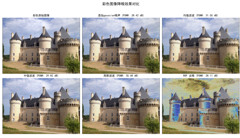
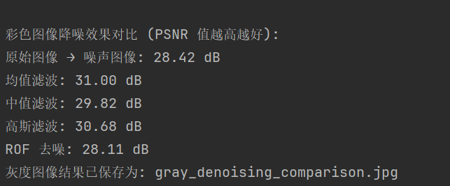
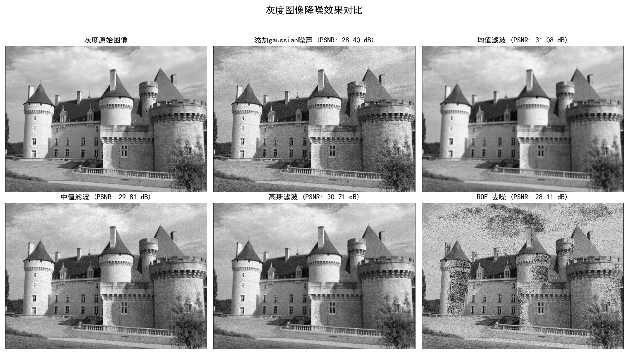
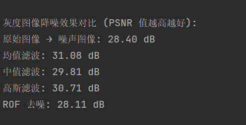
20.2椒盐噪声图像的降噪处理

import numpy as npimport matplotlib.pyplot as pltfrom PIL import Image, ImageFilter# 设置中文字体支持plt.rcParams[\"font.family\"] = [\"SimHei\"]plt.rcParams[\'axes.unicode_minus\'] = Falsedef add_noise(image, noise_type=\'gaussian\', amount=0.1): \"\"\"向图像添加噪声（支持彩色/灰度图像）\"\"\" img_array = np.array(image).astype(np.float32) is_color = len(img_array.shape) == 3 # 彩色图像为3通道（H,W,3） if noise_type == \'gaussian\': noise = np.random.normal(0, amount * 255, img_array.shape) noisy_img = np.clip(img_array + noise, 0, 255).astype(np.uint8) elif noise_type == \'salt_pepper\': noisy_img = img_array.copy() h, w = img_array.shape[:2] mask = np.random.rand(h, w) < amount # 噪声点掩码（H,W） if is_color: mask = np.stack([mask] * 3, axis=-1) # 扩展到3通道（H,W,3） # 随机分配盐（255）和椒（0）噪声 salt_mask = np.random.rand(*noisy_img[mask].shape)  tolerance: Uold = U.copy() # 计算梯度 GradUx = np.roll(U, -1, axis=1) - U # 水平梯度 GradUy = np.roll(U, -1, axis=0) - U # 垂直梯度 # 更新对偶变量 Px_new = Px + (tau / tv_weight) * GradUx Py_new = Py + (tau / tv_weight) * GradUy Norm_new = np.maximum(1, np.sqrt(Px_new ** 2 + Py_new ** 2)) # 避免除零 Px = Px_new / Norm_new Py = Py_new / Norm_new # 更新原始变量 RxPx = np.roll(Px, 1, axis=1) # 右移 RyPy = np.roll(Py, 1, axis=0) # 下移 DivP = (Px - RxPx) + (Py - RyPy) # 散度 U = Uold + tau * (DivP + image) # 计算误差 error = np.linalg.norm(U - Uold) / np.sqrt(U.size) return Udef rof_denoise_color(image_array): \"\"\"彩色图像ROF去噪（分通道处理，输入为（H,W,3）的uint8数组）\"\"\" h, w, c = image_array.shape if c != 3: raise ValueError(\"彩色图像必须为3通道\") denoised_channels = [] for channel in range(3): # 提取单通道并归一化到0-1 single_channel = image_array[:, :, channel].astype(np.float32) / 255.0 # ROF去噪 denoised = rof_denoise(single_channel, single_channel) # 裁剪到0-1范围，缩放回0-255，转为uint8 denoised = np.clip(denoised, 0, 1) denoised_channels.append((denoised * 255).astype(np.uint8)) # 堆叠为（H,W,3）的数组 denoised_array = np.stack(denoised_channels, axis=-1) # 确保形状正确（避免因图像太小导致的异常形状） if denoised_array.shape != (h, w, 3): raise RuntimeError(f\"彩色ROF去噪后形状异常：{denoised_array.shape}，预期：({h},{w},3)\") return denoised_arraydef demo_denoising(image_path, noise_type=\'gaussian\', amount=0.1, is_color=True): try: # 读取图像并确保格式正确 if is_color: original = Image.open(image_path).convert(\'RGB\') # 强制转为RGB模式（3通道） img_type = \"彩色\" output_suffix = f\"color_{noise_type}\" # 检查图像尺寸（避免过小图像） if original.size[0] < 3 or original.size[1] < 3: raise ValueError(\"图像尺寸过小，无法处理（至少3x3像素）\") else: original = Image.open(image_path).convert(\'L\') # 强制转为灰度模式（单通道） img_type = \"灰度\" output_suffix = f\"gray_{noise_type}\" if original.size[0] < 3 or original.size[1] < 3: raise ValueError(\"图像尺寸过小，无法处理（至少3x3像素）\") # 添加噪声 noisy = add_noise(original, noise_type, amount) # 传统滤波去噪 mean_denoised = mean_filter(noisy, size=3) median_denoised = median_filter(noisy, size=3) gaussian_denoised = gaussian_filter_pil(noisy, sigma=1.0) # ROF去噪 if is_color: # 转为数组（H,W,3） noisy_array = np.array(noisy) # 彩色ROF去噪 rof_denoised_array = rof_denoise_color(noisy_array) # 转为PIL图像（RGB模式） rof_denoised = Image.fromarray(rof_denoised_array, mode=\'RGB\') else: # 转为数组（H,W） noisy_array = np.array(noisy).astype(np.float32) / 255.0 # 归一化到0-1 # 灰度ROF去噪 rof_denoised_array = rof_denoise(noisy_array, noisy_array) # 处理为uint8的二维数组 rof_denoised_array = np.clip(rof_denoised_array, 0, 1) rof_denoised_array = (rof_denoised_array * 255).astype(np.uint8) # 确保是二维数组（避免多余维度） if len(rof_denoised_array.shape) == 3: rof_denoised_array = rof_denoised_array.squeeze() # 移除尺寸为1的维度 # 转为PIL图像（L模式） rof_denoised = Image.fromarray(rof_denoised_array, mode=\'L\') # 计算PSNR def psnr(original, processed): orig_arr = np.array(original) proc_arr = np.array(processed) mse = np.mean((orig_arr - proc_arr) ** 2) return 20 * np.log10(255.0 / np.sqrt(mse)) if mse != 0 else float(\'inf\') # 计算各指标 psnr_noisy = psnr(original, noisy) psnr_mean = psnr(original, mean_denoised) psnr_median = psnr(original, median_denoised) psnr_gaussian = psnr(original, gaussian_denoised) psnr_rof = psnr(original, rof_denoised) # 可视化 plt.figure(figsize=(15, 10)) plt.subplot(231) plt.title(f\'{img_type}原始图像\') plt.imshow(original, cmap=None if is_color else \'gray\') plt.axis(\'off\') plt.subplot(232) plt.title(f\'添加{noise_type}噪声 (PSNR: {psnr_noisy:.2f} dB)\') plt.imshow(noisy, cmap=None if is_color else \'gray\') plt.axis(\'off\') plt.subplot(233) plt.title(f\'均值滤波 (PSNR: {psnr_mean:.2f} dB)\') plt.imshow(mean_denoised, cmap=None if is_color else \'gray\') plt.axis(\'off\') plt.subplot(234) plt.title(f\'中值滤波 (PSNR: {psnr_median:.2f} dB)\') plt.imshow(median_denoised, cmap=None if is_color else \'gray\') plt.axis(\'off\') plt.subplot(235) plt.title(f\'高斯滤波 (PSNR: {psnr_gaussian:.2f} dB)\') plt.imshow(gaussian_denoised, cmap=None if is_color else \'gray\') plt.axis(\'off\') plt.subplot(236) plt.title(f\'ROF 去噪 (PSNR: {psnr_rof:.2f} dB)\') plt.imshow(rof_denoised, cmap=None if is_color else \'gray\') plt.axis(\'off\') # 保存与展示 plt.suptitle(f\'{img_type}图像{noise_type}噪声降噪对比\', fontsize=16) plt.tight_layout(rect=[0, 0, 1, 0.97]) output_path = f\'{output_suffix}_denoising.jpg\' plt.savefig(output_path, dpi=300) print(f\"{img_type}图像{noise_type}噪声结果已保存为: {output_path}\") plt.show() # 打印PSNR对比 print(f\"\\n{img_type}图像{noise_type}噪声降噪效果 (PSNR):\") print(f\"噪声图像: {psnr_noisy:.2f} dB\") print(f\"均值滤波: {psnr_mean:.2f} dB\") print(f\"中值滤波: {psnr_median:.2f} dB （推荐）\") print(f\"高斯滤波: {psnr_gaussian:.2f} dB\") print(f\"ROF去噪: {psnr_rof:.2f} dB\") except Exception as e: print(f\"处理出错: {e}\")if __name__ == \"__main__\": image_path = \"castle3.jpg\" # 确保该路径下有图像文件 noise_amount = 0.05 # 椒盐噪声比例（5%） # 1. 彩色图像 + 椒盐噪声处理 demo_denoising(image_path, noise_type=\'salt_pepper\', amount=noise_amount, is_color=True) # 2. 灰度图像 + 椒盐噪声处理 demo_denoising(image_path, noise_type=\'salt_pepper\', amount=noise_amount, is_color=False)

程序运行结果如下：

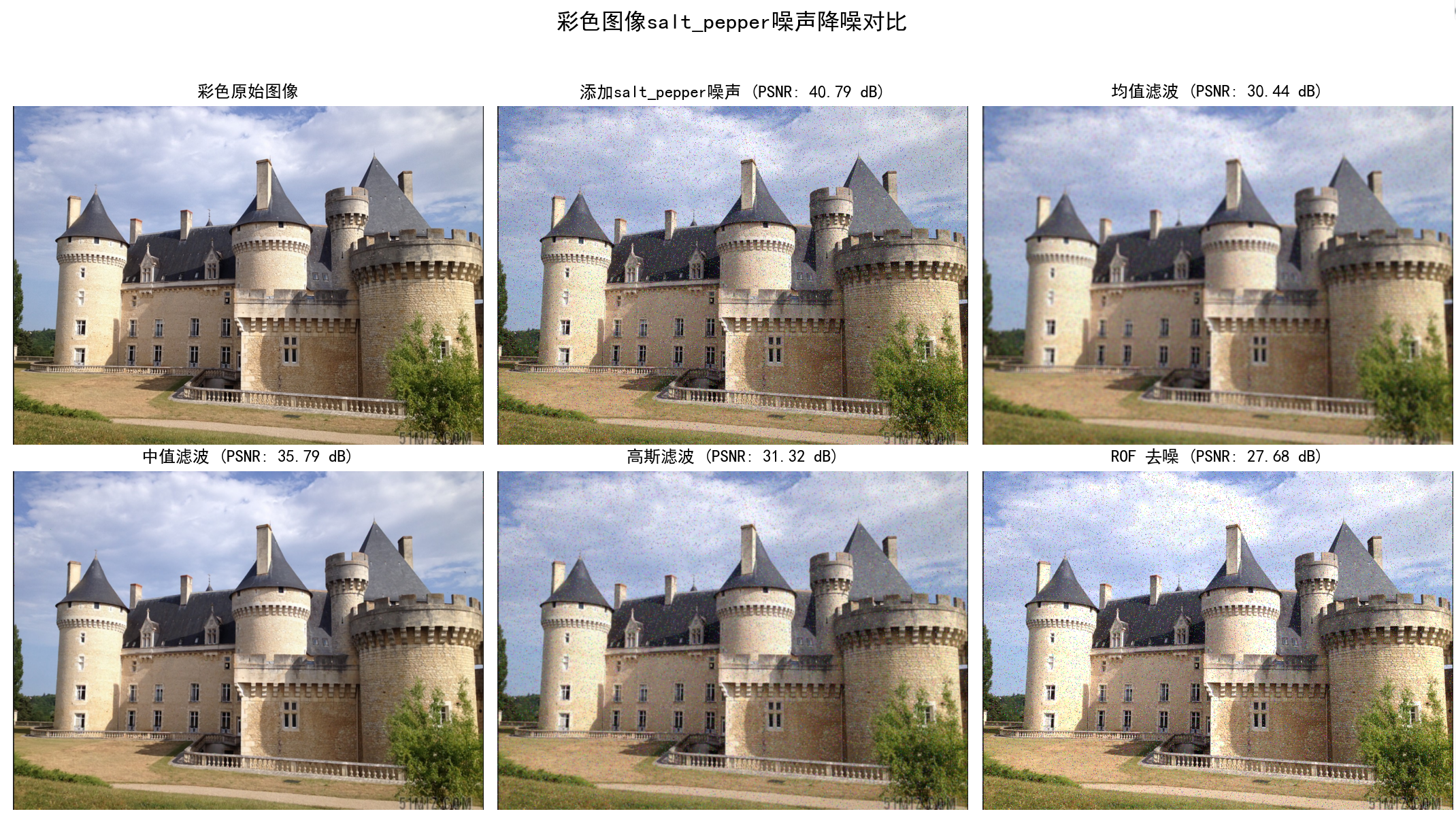
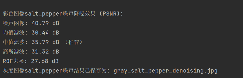
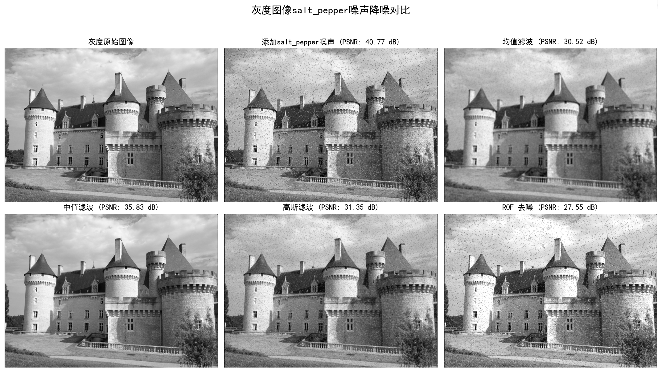
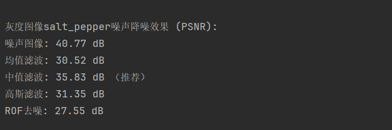
20.3对添加噪声的噪声实现降噪处理

import numpy as npfrom PIL import Imageimport matplotlib.pyplot as pltimport cv2import randomimport scipy.signalimport scipy.ndimage# 设置中文字体plt.rcParams[\'font.sans-serif\'] = [\'SimHei\']plt.rcParams[\'axes.unicode_minus\'] = False # 解决负号显示问题\"\"\"通用滤波函数\"\"\"def convert_2d(r): \"\"\"均值滤波（单通道）\"\"\" n = 3 window = np.ones((n, n)) / (n ** 2) return scipy.signal.convolve2d(r, window, mode=\'same\', boundary=\'symm\').astype(np.uint8)def process_color_channel(channel, noise_type=\'salt\'): \"\"\"处理单个彩色通道（添加噪声）\"\"\" rows, cols = channel.shape noisy_channel = channel.copy() if noise_type == \'salt\': # 椒盐噪声 snr = 0.9 noise_num = int((1 - snr) * rows * cols) for _ in range(noise_num): x = random.randint(0, rows - 1) y = random.randint(0, cols - 1) noisy_channel[x, y] = 0 if random.randint(0, 1) == 0 else 255 elif noise_type == \'gaussian\': # 高斯噪声 noise = np.random.normal(0, 48, (rows, cols)) # 均值0，标准差48 noisy_channel = np.clip(noisy_channel.astype(np.float32) + noise, 0, 255).astype(np.uint8) return noisy_channeldef color_median_filter(color_img, size=3): \"\"\"彩色图中值滤波（逐通道处理）\"\"\" r, g, b = cv2.split(color_img) r_filtered = scipy.ndimage.median_filter(r, size) g_filtered = scipy.ndimage.median_filter(g, size) b_filtered = scipy.ndimage.median_filter(b, size) return cv2.merge([r_filtered, g_filtered, b_filtered])def color_mean_filter(color_img): \"\"\"彩色图均值滤波（逐通道处理）\"\"\" r, g, b = cv2.split(color_img) r_filtered = convert_2d(r) g_filtered = convert_2d(g) b_filtered = convert_2d(b) return cv2.merge([r_filtered, g_filtered, b_filtered])\"\"\"灰度图处理（保留原有功能并优化）\"\"\"def process_gray_image(img_gray): # 添加椒盐噪声 gray_sp = img_gray.copy() rows, cols = gray_sp.shape snr = 0.9 noise_num = int((1 - snr) * rows * cols) for _ in range(noise_num): x = random.randint(0, rows - 1) y = random.randint(0, cols - 1) gray_sp[x, y] = 0 if random.randint(0, 1) == 0 else 255 # 添加高斯噪声 gray_gs = img_gray.copy() noise = np.random.normal(0, 48, (rows, cols)) gray_gs = np.clip(gray_gs.astype(np.float32) + noise, 0, 255).astype(np.uint8) # 滤波处理 gray_sp_mf = scipy.ndimage.median_filter(gray_sp, (3, 3)) # 中值滤波 gray_gs_mf = scipy.ndimage.median_filter(gray_gs, (3, 3)) gray_sp_me = convert_2d(gray_sp) # 均值滤波 gray_gs_me = convert_2d(gray_gs) return { \'original\': img_gray, \'salt\': gray_sp, \'gaussian\': gray_gs, \'salt_median\': gray_sp_mf, \'gaussian_median\': gray_gs_mf, \'salt_mean\': gray_sp_me, \'gaussian_mean\': gray_gs_me }\"\"\"彩色图处理（新增功能）\"\"\"def process_color_image(img_color): # 分离通道 r, g, b = cv2.split(img_color) # 为每个通道添加椒盐噪声 r_sp = process_color_channel(r, \'salt\') g_sp = process_color_channel(g, \'salt\') b_sp = process_color_channel(b, \'salt\') color_sp = cv2.merge([r_sp, g_sp, b_sp]) # 合并椒盐噪声通道 # 为每个通道添加高斯噪声 r_gs = process_color_channel(r, \'gaussian\') g_gs = process_color_channel(g, \'gaussian\') b_gs = process_color_channel(b, \'gaussian\') color_gs = cv2.merge([r_gs, g_gs, b_gs]) # 合并高斯噪声通道 # 滤波处理 color_sp_mf = color_median_filter(color_sp) # 椒盐噪声中值滤波 color_gs_mf = color_median_filter(color_gs) # 高斯噪声中值滤波 color_sp_me = color_mean_filter(color_sp) # 椒盐噪声均值滤波 color_gs_me = color_mean_filter(color_gs) # 高斯噪声均值滤波 return { \'original\': img_color, \'salt\': color_sp, \'gaussian\': color_gs, \'salt_median\': color_sp_mf, \'gaussian_median\': color_gs_mf, \'salt_mean\': color_sp_me, \'gaussian_mean\': color_gs_me }\"\"\"显示对比结果\"\"\"def show_comparison(gray_results, color_results): # 创建画布（2行8列，展示灰度和彩色的所有结果） plt.figure(figsize=(20, 10)) # 第一行：灰度图结果 plt.subplot(2, 8, 1) plt.title(\'灰度原图\') plt.imshow(gray_results[\'original\'], cmap=\'gray\') plt.axis(\'off\') plt.subplot(2, 8, 2) plt.title(\'灰度椒盐噪声\') plt.imshow(gray_results[\'salt\'], cmap=\'gray\') plt.axis(\'off\') plt.subplot(2, 8, 3) plt.title(\'灰度高斯噪声\') plt.imshow(gray_results[\'gaussian\'], cmap=\'gray\') plt.axis(\'off\') plt.subplot(2, 8, 4) plt.title(\'椒盐-中值滤波\') plt.imshow(gray_results[\'salt_median\'], cmap=\'gray\') plt.axis(\'off\') plt.subplot(2, 8, 5) plt.title(\'高斯-中值滤波\') plt.imshow(gray_results[\'gaussian_median\'], cmap=\'gray\') plt.axis(\'off\') plt.subplot(2, 8, 6) plt.title(\'椒盐-均值滤波\') plt.imshow(gray_results[\'salt_mean\'], cmap=\'gray\') plt.axis(\'off\') plt.subplot(2, 8, 7) plt.title(\'高斯-均值滤波\') plt.imshow(gray_results[\'gaussian_mean\'], cmap=\'gray\') plt.axis(\'off\') # 第二行：彩色图结果 plt.subplot(2, 8, 9) plt.title(\'彩色原图\') plt.imshow(cv2.cvtColor(color_results[\'original\'], cv2.COLOR_BGR2RGB)) # 转换为RGB显示 plt.axis(\'off\') plt.subplot(2, 8, 10) plt.title(\'彩色椒盐噪声\') plt.imshow(cv2.cvtColor(color_results[\'salt\'], cv2.COLOR_BGR2RGB)) plt.axis(\'off\') plt.subplot(2, 8, 11) plt.title(\'彩色高斯噪声\') plt.imshow(cv2.cvtColor(color_results[\'gaussian\'], cv2.COLOR_BGR2RGB)) plt.axis(\'off\') plt.subplot(2, 8, 12) plt.title(\'椒盐-中值滤波\') plt.imshow(cv2.cvtColor(color_results[\'salt_median\'], cv2.COLOR_BGR2RGB)) plt.axis(\'off\') plt.subplot(2, 8, 13) plt.title(\'高斯-中值滤波\') plt.imshow(cv2.cvtColor(color_results[\'gaussian_median\'], cv2.COLOR_BGR2RGB)) plt.axis(\'off\') plt.subplot(2, 8, 14) plt.title(\'椒盐-均值滤波\') plt.imshow(cv2.cvtColor(color_results[\'salt_mean\'], cv2.COLOR_BGR2RGB)) plt.axis(\'off\') plt.subplot(2, 8, 15) plt.title(\'高斯-均值滤波\') plt.imshow(cv2.cvtColor(color_results[\'gaussian_mean\'], cv2.COLOR_BGR2RGB)) plt.axis(\'off\') plt.tight_layout() plt.savefig(\'noise_reduction_processing_castle3.jpg\') plt.show()def main(): # 读取图片（确保路径正确） img_path = \'castle3.jpg\' img_color = cv2.imread(img_path) # 读取彩色图（BGR格式） img_gray = cv2.cvtColor(img_color, cv2.COLOR_BGR2GRAY) # 转换为灰度图 # 处理灰度图和彩色图 gray_results = process_gray_image(img_gray) color_results = process_color_image(img_color) # 显示对比结果 show_comparison(gray_results, color_results)if __name__ == \'__main__\': main()

程序运行结果如下：

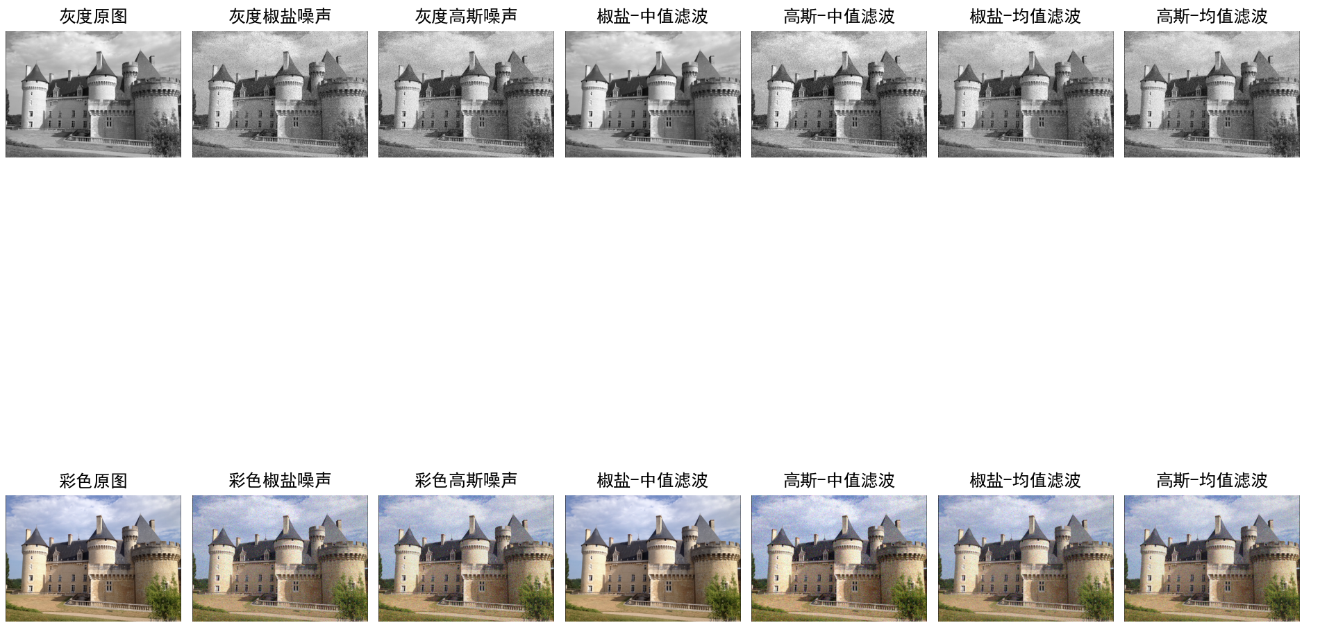
20.4噪声图像的降噪处理

import numpy as npimport matplotlib.pyplot as pltfrom PIL import Image, ImageFilter# 设置中文字体支持plt.rcParams[\"font.family\"] = [\"SimHei\"]plt.rcParams[\'axes.unicode_minus\'] = Falsedef add_noise(image, noise_type=\'gaussian\', amount=0.1): \"\"\"向图像添加噪声（修复数据类型问题）\"\"\" img_array = np.array(image, dtype=np.uint8) # 强制为uint8 is_color = len(img_array.shape) == 3 if noise_type == \'gaussian\': # 高斯噪声：先转为float计算，再转回uint8 noise = np.random.normal(0, amount * 255, img_array.shape).astype(np.float32) noisy_img = np.clip(img_array.astype(np.float32) + noise, 0, 255).astype(np.uint8) elif noise_type == \'salt_pepper\': # 椒盐噪声：直接在uint8上操作 noisy_img = img_array.copy() h, w = img_array.shape[:2] mask = np.random.rand(h, w) < amount if is_color: mask = np.stack([mask] * 3, axis=-1) # 确保噪声值为uint8类型 salt = np.where(np.random.rand(*noisy_img[mask].shape)  tolerance: Uold = U.copy() GradUx = np.roll(U, -1, axis=1) - U GradUy = np.roll(U, -1, axis=0) - U Px_new = Px + (tau / tv_weight) * GradUx Py_new = Py + (tau / tv_weight) * GradUy Norm_new = np.maximum(1, np.sqrt(Px_new ** 2 + Py_new ** 2)) Px = Px_new / Norm_new Py = Py_new / Norm_new RxPx = np.roll(Px, 1, axis=1) RyPy = np.roll(Py, 1, axis=0) DivP = (Px - RxPx) + (Py - RyPy) U = Uold + tau * (DivP + image) error = np.linalg.norm(U - Uold) / np.sqrt(U.size) return U # 返回float32，后续需转换为uint8def rof_denoise_color(image_array): \"\"\"彩色ROF去噪（确保输出为uint8的RGB模式）\"\"\" denoised_channels = [] for channel in range(3): single_channel = image_array[:, :, channel].astype(np.float32) / 255.0 denoised = rof_denoise(single_channel, single_channel) # 关键修复：将float32转为uint8（0-255） denoised_uint8 = (np.clip(denoised, 0, 1) * 255).astype(np.uint8) denoised_channels.append(denoised_uint8) # 确保输出形状为(H, W, 3)，数据类型uint8 return np.stack(denoised_channels, axis=-1)def psnr(original, processed): orig_arr = np.array(original, dtype=np.float32) proc_arr = np.array(processed, dtype=np.float32) mse = np.mean((orig_arr - proc_arr) ** 2) return 20 * np.log10(255.0 / np.sqrt(mse)) if mse != 0 else float(\'inf\')def demo_denoising(image_path, noise_types=[\'gaussian\', \'salt_pepper\'], amounts=[0.1, 0.05], is_color=True): try: # 读取图像时明确指定模式，避免模式错误 if is_color: original = Image.open(image_path).convert(\'RGB\') # 强制RGB模式 img_type = \"彩色\" output_suffix = \"color\" else: original = Image.open(image_path).convert(\'L\') # 强制灰度模式 img_type = \"灰度\" output_suffix = \"gray\" results = {} for noise_type, amount in zip(noise_types, amounts): noisy = add_noise(original, noise_type, amount) # 滤波处理（输出为PIL图像，模式正确） mean_denoised = mean_filter(noisy, size=3) median_denoised = median_filter(noisy, size=3) gaussian_denoised = gaussian_filter_pil(noisy, sigma=1.0) # ROF去噪（修复数据类型转换） if is_color: noisy_array = np.array(noisy, dtype=np.uint8) # 确保输入为uint8 rof_denoised_array = rof_denoise_color(noisy_array) # 明确指定模式为RGB，避免自动检测错误 rof_denoised = Image.fromarray(rof_denoised_array, mode=\'RGB\') else: noisy_array = np.array(noisy, dtype=np.uint8) / 255.0 rof_denoised_float = rof_denoise(noisy_array, noisy_array) # 转换为uint8并指定灰度模式\'L\' rof_denoised_uint8 = (np.clip(rof_denoised_float, 0, 1) * 255).astype(np.uint8) rof_denoised = Image.fromarray(rof_denoised_uint8, mode=\'L\') # 计算PSNR results[noise_type] = { \'noisy\': noisy, \'mean\': mean_denoised, \'median\': median_denoised, \'gaussian\': gaussian_denoised, \'rof\': rof_denoised, \'psnr\': {  \'noisy\': psnr(original, noisy),  \'mean\': psnr(original, mean_denoised),  \'median\': psnr(original, median_denoised),  \'gaussian\': psnr(original, gaussian_denoised),  \'rof\': psnr(original, rof_denoised) } } # 计算所需子图数量（1张原图 + 每种噪声5张图：噪声图+4种去噪结果） n_noise = len(noise_types) total_plots = 1 + n_noise * 5 fig, axes = plt.subplots(2, (total_plots + 1) // 2, figsize=(24, 8)) # 自动调整列数 axes = axes.flatten()[:total_plots] # 只保留需要的子图 # 原始图像 axes[0].set_title(f\'{img_type}原始图像\') axes[0].imshow(original, cmap=None if is_color else \'gray\') axes[0].axis(\'off\') # 噪声和降噪结果（确保每种噪声的5张图连续显示） plot_idx = 1 for noise_type in noise_types: res = results[noise_type] # 噪声图像 axes[plot_idx].set_title(f\'{noise_type}噪声\\nPSNR: {res[\"psnr\"][\"noisy\"]:.2f} dB\') axes[plot_idx].imshow(res[\'noisy\'], cmap=None if is_color else \'gray\') axes[plot_idx].axis(\'off\') plot_idx += 1 # 均值滤波（确保高斯噪声的均值滤波图显示） axes[plot_idx].set_title(f\'{noise_type}噪声-均值滤波\\nPSNR: {res[\"psnr\"][\"mean\"]:.2f}\') axes[plot_idx].imshow(res[\'mean\'], cmap=None if is_color else \'gray\') axes[plot_idx].axis(\'off\') plot_idx += 1 # 中值滤波 axes[plot_idx].set_title(f\'{noise_type}噪声-中值滤波\\nPSNR: {res[\"psnr\"][\"median\"]:.2f}\') axes[plot_idx].imshow(res[\'median\'], cmap=None if is_color else \'gray\') axes[plot_idx].axis(\'off\') plot_idx += 1 # 高斯滤波 axes[plot_idx].set_title(f\'{noise_type}噪声-高斯滤波\\nPSNR: {res[\"psnr\"][\"gaussian\"]:.2f}\') axes[plot_idx].imshow(res[\'gaussian\'], cmap=None if is_color else \'gray\') axes[plot_idx].axis(\'off\') plot_idx += 1 # ROF去噪 axes[plot_idx].set_title(f\'{noise_type}噪声-ROF去噪\\nPSNR: {res[\"psnr\"][\"rof\"]:.2f}\') axes[plot_idx].imshow(res[\'rof\'], cmap=None if is_color else \'gray\') axes[plot_idx].axis(\'off\') plot_idx += 1 plt.suptitle(f\'{img_type}图像噪声对比\', fontsize=16) plt.tight_layout(rect=[0, 0, 1, 0.95]) output_path = f\'{output_suffix}_noise_comparison.jpg\' plt.savefig(output_path, dpi=300) print(f\"{img_type}图像结果已保存至: {output_path}\") plt.show() # 打印PSNR for noise_type, res in results.items(): print(f\"\\n{img_type}图像{noise_type}噪声降噪效果:\") print(f\"噪声图像: {res[\'psnr\'][\'noisy\']:.2f} dB\") print(f\"均值滤波: {res[\'psnr\'][\'mean\']:.2f} dB\") print(f\"中值滤波: {res[\'psnr\'][\'median\']:.2f} dB\") print(f\"高斯滤波: {res[\'psnr\'][\'gaussian\']:.2f} dB\") print(f\"ROF去噪: {res[\'psnr\'][\'rof\']:.2f} dB\") except Exception as e: print(f\"处理出错: {e}\")if __name__ == \"__main__\": image_path = \"castle3.jpg\" # 彩色图像处理 demo_denoising(image_path, [\'gaussian\', \'salt_pepper\'], [0.1, 0.05], is_color=True) # 灰度图像处理 demo_denoising(image_path, [\'gaussian\', \'salt_pepper\'], [0.1, 0.05], is_color=False)

程序运行结果如下：

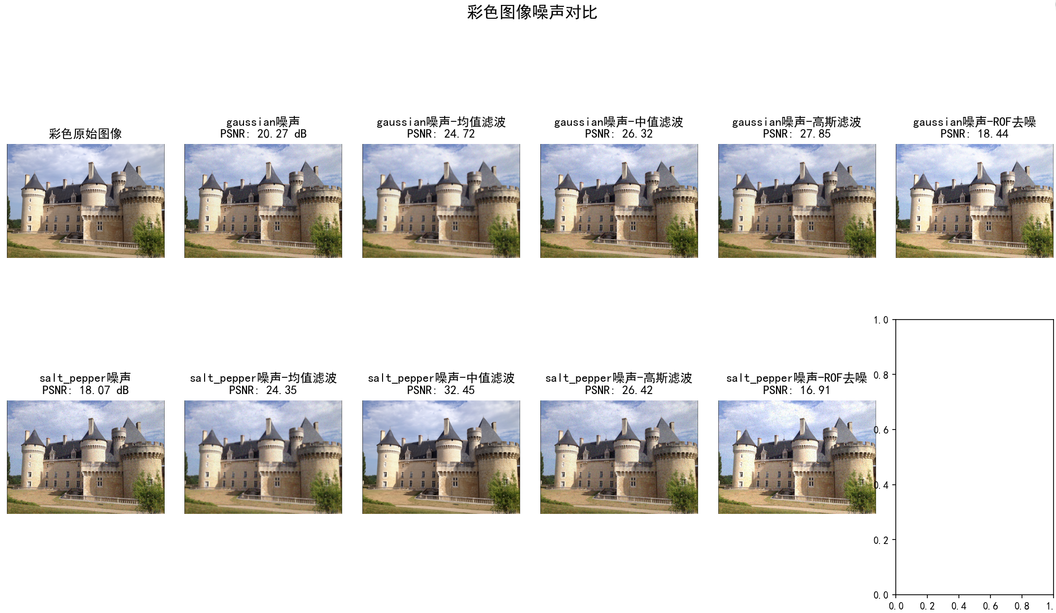
彩色图像gaussian噪声降噪效果:
噪声图像: 20.27 dB
均值滤波: 24.72 dB
中值滤波: 26.32 dB
高斯滤波: 27.85 dB
ROF去噪: 18.44 dB

彩色图像salt_pepper噪声降噪效果:
噪声图像: 18.07 dB
均值滤波: 24.35 dB
中值滤波: 32.45 dB
高斯滤波: 26.42 dB
ROF去噪: 16.91 dB
灰度图像结果已保存至: gray_noise_comparison.jpg

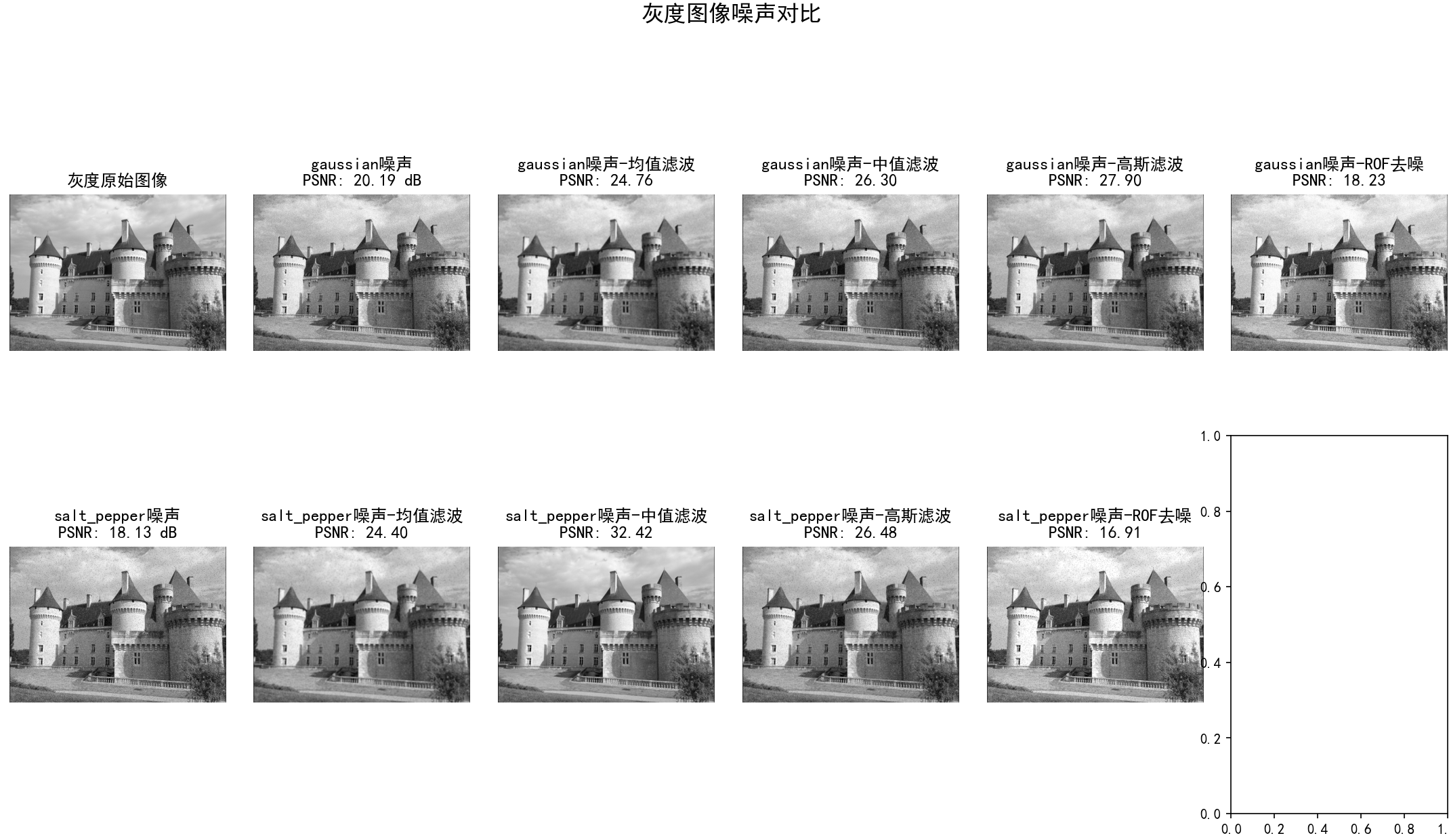
灰度图像gaussian噪声降噪效果:
噪声图像: 20.19 dB
均值滤波: 24.76 dB
中值滤波: 26.30 dB
高斯滤波: 27.90 dB
ROF去噪: 18.23 dB

灰度图像salt_pepper噪声降噪效果:
噪声图像: 18.13 dB
均值滤波: 24.40 dB
中值滤波: 32.42 dB
高斯滤波: 26.48 dB
ROF去噪: 16.91 dB

三、总结

本文介绍了计算机视觉编程中常用的图像处理技术，涵盖基础库操作、图像变换、特征分析、降噪处理等多个方面。主要内容包括：

基础库使用：NumPy数组操作、SciPy科学计算、Pandas数据分析和PIL图像处理库的基本用法。
图像处理技术：

格式转换与基本操作（裁剪、缩放、旋转）
灰度/彩色图像变换（反向、亮度调整、伽马校正）
直方图均衡化与主成分分析
边缘检测（Sobel算子、高斯导数）
形态学处理（二值化、连通区域分析）

3.高级应用：

图像降噪（高斯/椒盐噪声处理）
图像去雾算法
交互式图像标注
多尺度特征分析

4.可视化方法：通过对比图直观展示不同处理效果，分析PSNR/SSIM等质量指标。

文中提供了完整的Python代码示例和运行结果，展示了从基础操作到高级算法的完整计算机视觉处理流程。这些技术可应用于图像增强、目标检测、特征提取等多个领域。

猎鲲钓鱼部落

计算机视觉编程基础知识

一、本文计算机视觉编程可能用到的图像

二、计算机视觉编程基础知识

三、总结

公告

DeepSeek全套部署资料免费下载

免费可商用字体批量下载

标签

计算机视觉编程基础知识

一、本文计算机视觉编程可能用到的图像

二、计算机视觉编程基础知识

三、总结

相关问题

公告

DeepSeek全套部署资料免费下载

免费可商用字体批量下载

标签