NLP学习系列 | Transformer代码简单实现

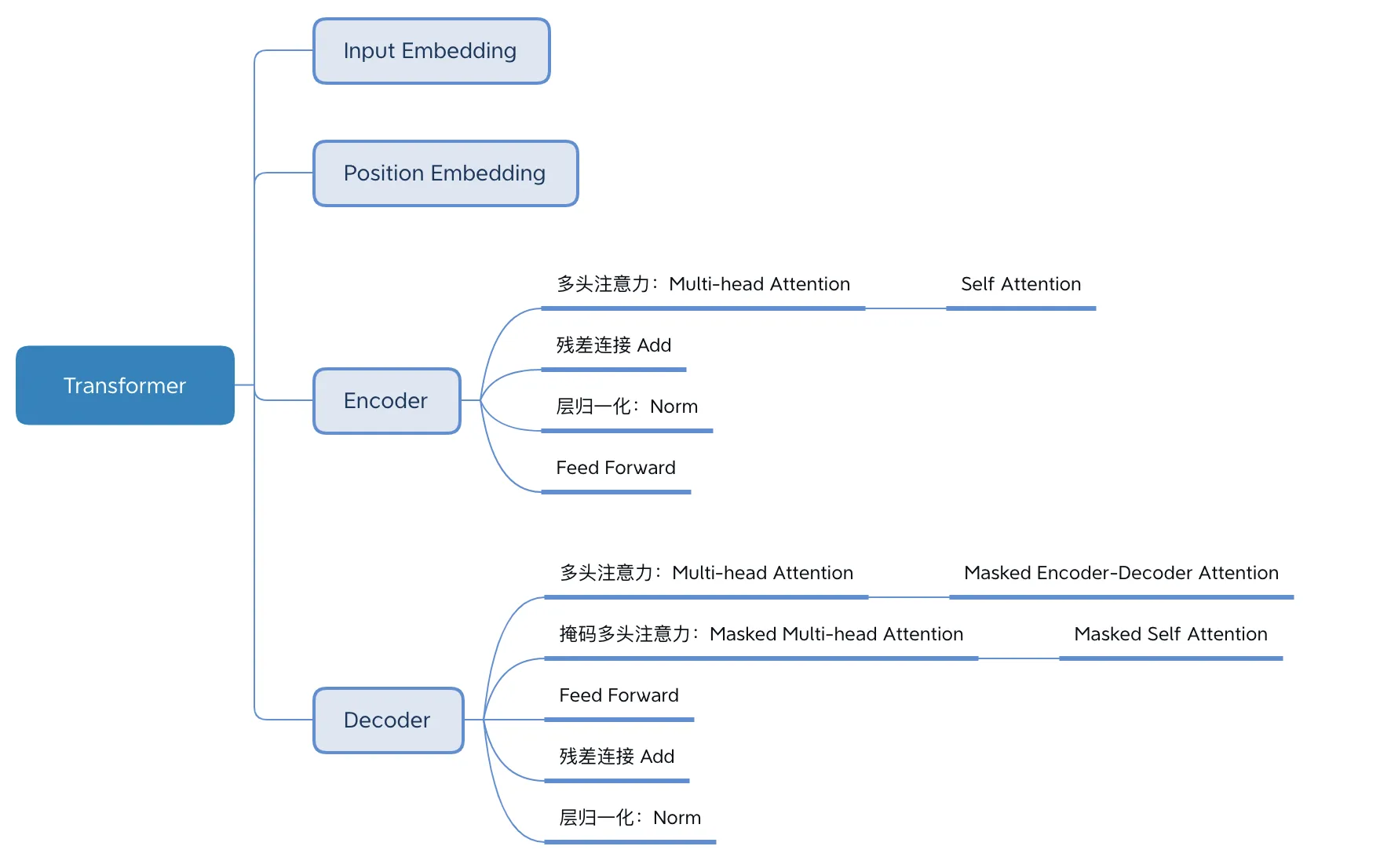
Transformer模型最初是在 2017 年的论文《Attention is all you need》中提出的，并用于机器翻译任务，和以往网络架构有所区别的是，该网络架构中，编码器和解码器没有采用 RNN 或 CNN 等网络架构，而是采用完全依赖于注意力机制的架构。架构如下所示 :

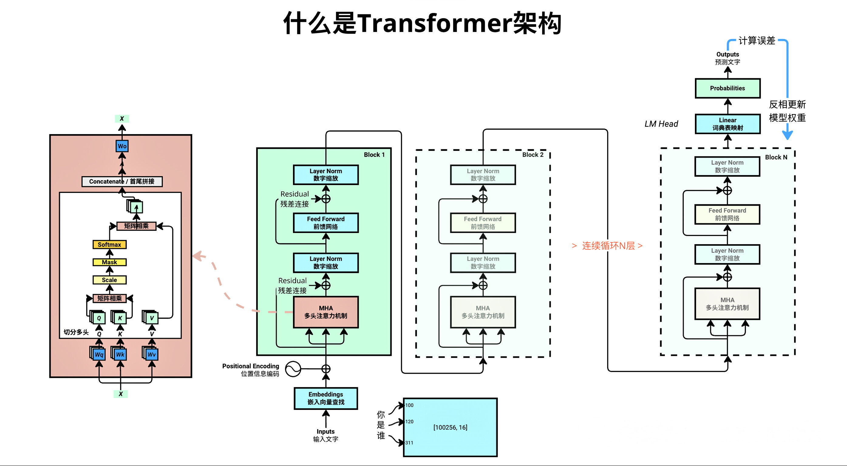
下面跟着我一起用代码来熟悉Transformer的架构,相信你会有收获, 毕竟实践出真知.

1、设置超参数

import osimport requestsimport matplotlib.pyplot as pltimport mathimport tiktokenimport torchimport torch.nn as nn

超参数是模型的外部配置，无法在训练过程中从数据中学习到。它们在训练过程开始前设置，在控制训练算法的行为和训练后模型的性能方面起着至关重要的作用。

batch_size = 4 #每批样本的数量context_length = 16 #上下文长度，指每个样本中包含的 token 序列长度（比如文本中的字符数、单词数）d_model = 64 # 词嵌入（token embeddings）的向量维度num_layers = 8 # Transformer块的数量num_heads = 4 # 多头注意力机制中的“头数” # 我们的代码中通过 d_model / num_heads = 来获取 head_sizelearning_rate = 1e-3 # 学习率，控制模型参数更新的步长 0.001dropout = 0.1 # Dropout比率，训练时随机将 10% 的神经元输出设为 0，用于防止模型过拟合max_iters = 5000 #总的训练迭代次数，即模型会进行 5000 次参数更新eval_interval = 50 #模型评估的频率，每训练 50 次迭代后，会对模型性能（通常是损失值）进行一次评估eval_iters = 20 #评估时计算损失的迭代次数。为了使评估结果更稳定，会取 20 次迭代的损失平均值作为评估指标device = torch.device(\"mps\" if torch.backends.mps.is_available() else \"cpu\") #设置GPU训练,mac M1芯片# device = \'cuda\' if torch.cuda.is_available() else \'cpu\' # WindowsTORCH_SEED = 1337 #固定 PyTorch 的随机数生成器种子torch.manual_seed(TORCH_SEED)

2、准备数据集

从huggingface社区下载一个 [https://huggingface.co/datasets/goendalf666/sales-textbook_for_convincing_and_selling/raw/main/sales_textbook.txt ]

current_working_dir = os.getcwd()print(\"当前工作目录:\", current_working_dir)if not os.path.exists(\'sales_textbook.txt\'): url = \'https://huggingface.co/datasets/goendalf666/sales-textbook_for_convincing_and_selling/raw/main/sales_textbook.txt\' with open(\'sales_textbook.txt\', \'w\') as f: f.write(requests.get(url).text)with open(\'sales_textbook.txt\', \'r\', encoding=\'utf-8\') as f: text = f.read()

当前工作目录: /Users/thinkinspure/PycharmProjects/MyPython/ai/Week6

3、实现Transformer

3.1、分词(Tokenization)

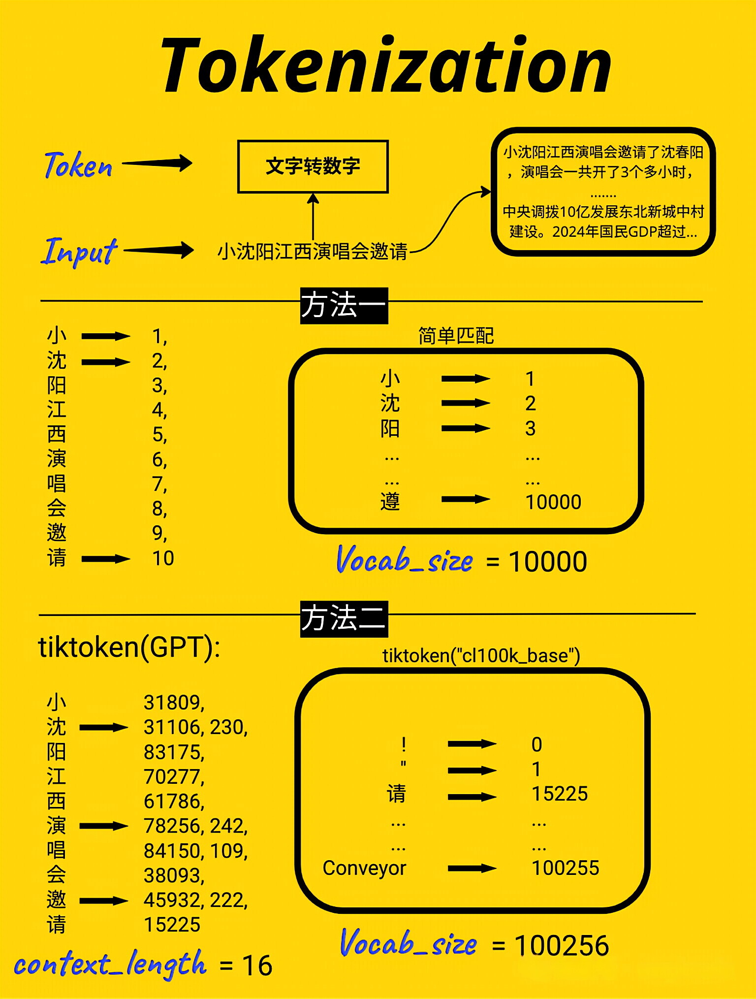
将原始文本转换为模型可处理的数字token张量，并获取token序列的基本信息（长度、最大索引），为后续模型训练做准备

encoding = tiktoken.get_encoding(\"cl100k_base\") #我们将使用tiktoken库(OpenAI开发的高效分词库)对数据集进行分词tokenized_text = encoding.encode(text) #使用上面初始化的分词器对原始文本（text，即之前读取的 sales_textbook.txt 内容）进行编码tokenized_text = torch.tensor(tokenized_text, dtype=torch.long, device=device) #将token序列转换为PyTorch张量max_token_value = tokenized_text.max().item() #计算token序列中的最大整数值print(f\"输出分词后的 token 总数: {len(tokenized_text)}\")print(f\"输出最大token值: {max_token_value}\")

输出分词后的 token 总数: 77919输出最大token值: 100069

打印encode结果,注意某些单词会对应多个token

print(encoding.encode(\'Chapter 1: Building Rapport and Capturing\'))print(encoding.decode([26072, 220, 16, 25, 17283, 23097, 403, 323, 17013, 1711])) # \"Rapport\" is tokenized as two tokens: \"Rap\"[23097] and \"port\"[403]print(encoding.decode([1383, 88861, 279,1989, 315, 25607, 16940, 65931, 323, 32097, 11, 584, 26458, 13520, 449]))

[26072, 220, 16, 25, 17283, 23097, 403, 323, 17013, 1711]Chapter 1: Building Rapport and CapturingBy mastering the art of identifying underlying motivations and desires, we equip ourselves with

3.2、词嵌入(Word Embedding)

把数据集分为训练集和验证集。训练集将用于训练模型，验证集将用于评估模型的性能

# 划分训练集和验证集 8:2split_idx = int(len(tokenized_text) * 0.8)train_data = tokenized_text[:split_idx]val_data = tokenized_text[split_idx:]

# 为训练批次准备数据data = train_dataidxs = torch.randint(low=0, high=len(data) - context_length, size=(batch_size,)) #生成batch_size个随机起始索引，用于从train_data中截取训练样本x_batch = torch.stack([data[idx:idx + context_length] for idx in idxs]).to(device) #构造模型的输入批次（x_batch），每个样本是context_length长度的 token 序列y_batch = torch.stack([data[idx + 1:idx + context_length + 1] for idx in idxs]).to(device)#对应输入x_batch的 “下一个 token 序列”（用于计算预测损失）print(x_batch.shape, y_batch.shape)

torch.Size([4, 16]) torch.Size([4, 16])

import pandas as pdpd.set_option(\'display.expand_frame_repr\', False)print(\"x_batch:\\n\", pd.DataFrame(x_batch.data.detach().cpu().numpy())) #转换为 pandas 的 DataFrame 格式

x_batch: 0 1 2 3 4 5 6 7 8 9 10 11 12 13 14 150 7528 4325 11 5557 706 3719 459 26154 961 315 1057 6439 11 2737 279 21151 323 43010 2592 315 2038 627 10673 306 13071 4726 1946 1392 100039 555 23537 67632 596 16024 11 1977 39474 11 323 6106 814 527 389 279 1890 2199 13 17893 19407 5376 279 17393 315 15676 264 6412 627 22 13 9356 287 4761 25593 323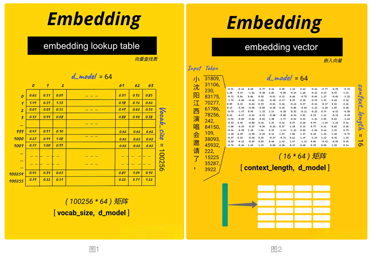

# 定义一个 Token 嵌入查找表(Token Embedding look-up table), 见图1token_embedding_lookup_table = nn.Embedding(max_token_value+1, d_model).to(device)print(\"Token Embedding Look-up table: \", token_embedding_lookup_table)# 获取x、y的embedding, 见图2x_batch_embedding = token_embedding_lookup_table(x_batch.data) # [4, 16, 64] [batch_size, context_length, d_model]y_batch_embedding = token_embedding_lookup_table(y_batch.data)x_batch_embedding.shape, y_batch_embedding.shape

Token Embedding Look-up table: Embedding(100070, 64)(torch.Size([4, 16, 64]), torch.Size([4, 16, 64]))

3.3、位置编码(Positional Encoding)

Transformer模型中经典的正弦余弦位置编码（Sinusoidal Position Encoding），用于向模型注入序列中 token 的位置信息（因为Transformer的自注意力机制本身不包含位置感知能力）, 简单说就是给数字加位置, 解决以下三个问题 :

• 每个单词token包含它的位置信息
• 模型可看到文字间“距离”
• 模型可看懂并学习到位置编码的规则

这个位置向量的具体计算方法有很多种，论文中的计算方法如下 :

PE(pos,2i)=sin(pos/10000^2i /d_model )

PE(pos,2i+1)= cos(pos/10000^2i /d_model )

其中 pos 是指当前词在句子中的位置， i 是指向量中每个值的 index ，可以看出，在偶数位置，使用正弦编码，在奇数位置，使用余弦编码

对应下面代码中的div_term, 和 position_encoding_lookup_table (见图3)

要注意一个点 , 位置编码 (position_encoding_lookup_table) 不会随着模型训练而发生变化 ! !

词嵌入向量会随着训练发生变化(x_batch_embedding、y_batch_embedding)

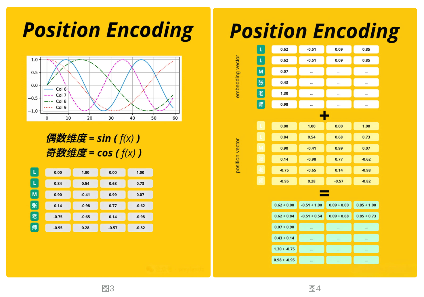
# 定义一个位置编码查找表 (Position Encoding look-up table)# 实现了Transformer模型中经典的正弦余弦位置编码（Sinusoidal Position Encoding）position_encoding_lookup_table = torch.zeros(context_length, d_model).to(device) #初始化一个位置编码表,后续填充position = torch.arange(0, context_length, dtype=torch.float).unsqueeze(1) #生成 “位置索引” 张量div_term = torch.exp(torch.arange(0, d_model, 2).float() * (-math.log(10000.0) / d_model))position_encoding_lookup_table[:, 0::2] = torch.sin(position * div_term)position_encoding_lookup_table[:, 1::2] = torch.cos(position * div_term)position_encoding_lookup_table = position_encoding_lookup_table.unsqueeze(0).expand(batch_size, -1, -1) #add batch dimensionprint(\"Position Encoding Look-up Table: \", position_encoding_lookup_table.shape) # [4, 16, 64] [batch_size, context_length, d_model]pd.DataFrame(position_encoding_lookup_table[0].detach().cpu().numpy())

Position Encoding Look-up Table: torch.Size([4, 16, 64])

将 Transformer 中的位置编码（Positional Encoding）以热图（Heatmap）的形式可视化

def visualize_pe(pe): plt.imshow(pe, aspect=\"auto\") # 绘制热图 plt.title(\"Positional Encoding\") # 设置标题 plt.xlabel(\"Encoding Dimension\") # x轴标签：编码维度（d_model） plt.ylabel(\"Position Index\") # y轴标签：位置索引（0到context_length-1） plt.colorbar() # 添加颜色条（表示数值大小与颜色的对应关系） plt.show() # 显示图像# 提取第一个样本的位置编码，转移到CPU并转换为numpy数组position_encoding_lookup_table2_np = position_encoding_lookup_table[0].cpu().numpy()visualize_pe(position_encoding_lookup_table2_np)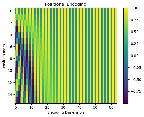

# 将位置编码添加到输入嵌入向量中 (见图4)input_embedding_x = x_batch_embedding + position_encoding_lookup_table # [4, 16, 64] [batch_size, context_length, d_model]input_embedding_y = y_batch_embedding + position_encoding_lookup_tablepd.DataFrame(input_embedding_x[0].detach().cpu().numpy())

见图4, 结果自行输出查看

3.4、Transformer Block

3.4.1、图解softmax

讲这个之前,先看下下面softmax图, 理解下基本概念

下面就到大名鼎鼎的多头注意力机制了, 大家注意先仔细查看图 , 然后再结合代码进行查看, 会有不一样的理解 , 让我们一起慢慢探索 

3.4.2、输入生成 Q/K/V

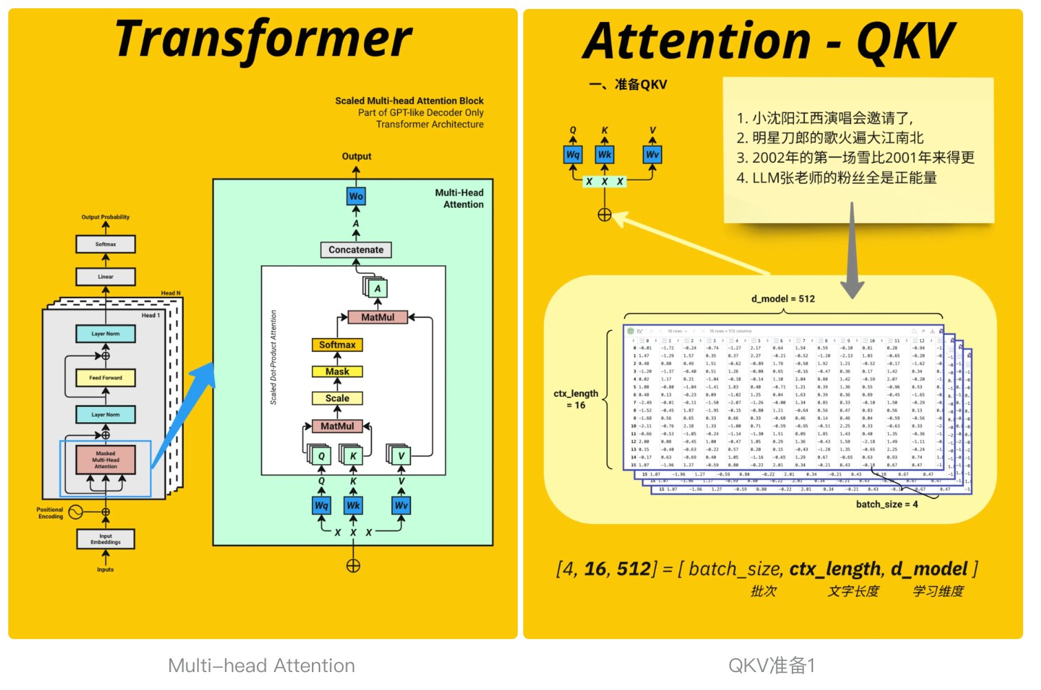
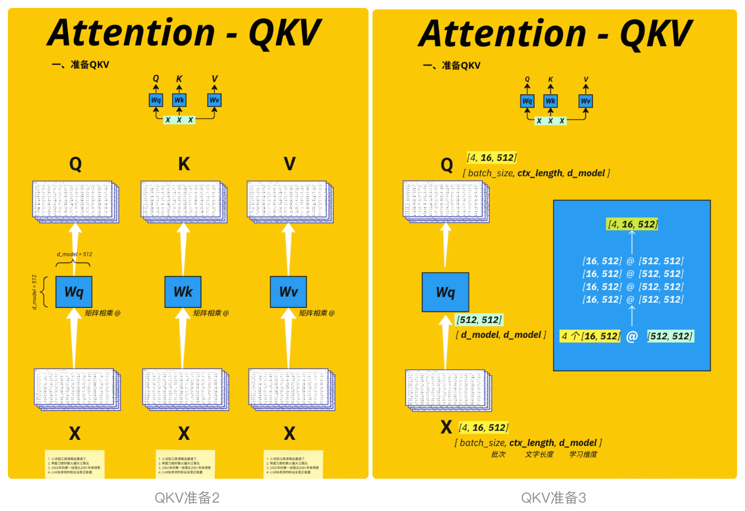
# Prepare Query, Key, Value for Multi-head AttentionX = input_embedding_x #见图QKV准备1, 忽略d_model(可设置)query = key = value = X # [4, 16, 64] [batch_size, context_length, d_model]query.shape

torch.Size([4, 16, 64]) 

3.4.3、多头切分

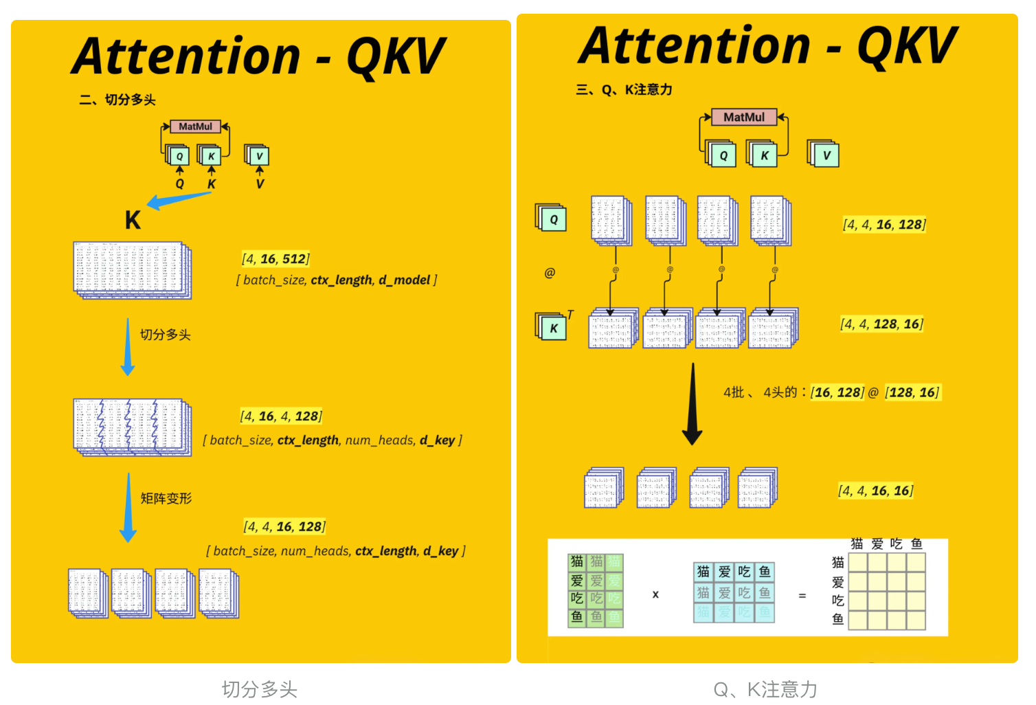
将单个注意力机制拆分为多个并行的 \"子注意力机制\"（即多头），让模型同时捕捉不同类型的关联关系（例如有的头关注语法，有的头关注语义）

• 通过线性变换将输入转换为 Q/K/V 向量；
• 将 Q/K/V 拆分为多个并行的注意力头，每个头独立计算注意力权重，最终再合并结果
• #见图 切分多头

# Define Query, Key, Value weight matricesWq = nn.Linear(d_model, d_model).to(device) # Query的权重矩阵Wk = nn.Linear(d_model, d_model).to(device) # Key的权重矩阵Wv = nn.Linear(d_model, d_model).to(device) # Value的权重矩阵#切分多头,核心逻辑 # 将Q切分为多头：从[4,16,64] → [4,16,4,16]Q = Wq(query) #[4, 16, 64]Q = Q.view(batch_size, -1, num_heads, d_model // num_heads) #[4, 16, 4, 16]# K、V同理K = Wk(key) #[4, 16, 64]K = K.view(batch_size, -1, num_heads, d_model // num_heads) #[4, 16, 4, 16]V = Wv(value) #[4, 16, 64]V = V.view(batch_size, -1, num_heads, d_model // num_heads) #[4, 16, 4, 16]#print(torch.round(Q[0] * 100) / 100)qqq = Q.detach().cpu().numpy()#for qs in qqq: #for qss in qs: #print(pd.DataFrame(qss))print(Q.shape) # [4, 16, 4, 16] [batch_size, context_length, num_heads, head_size]

torch.Size([4, 16, 4, 16])

下面的代码是为了调整 Query (Q)、Key (K)、Value (V) 的维度顺序，为后续计算多头注意力权重做准备。转置操作看似简单，却是多头注意力机制中保证矩阵乘法维度匹配的关键步骤

# Transpose q,k,v from [batch_size, context_length, num_heads, head_size] to [batch_size, num_heads, context_length, head_size]# 见图 切分多头 过程# num_heads 这里后面不参与具体运算Q = Q.transpose(1, 2) # [4, 4, 16, 16]K = K.transpose(1, 2) # [4, 4, 16, 16]V = V.transpose(1, 2) # [4, 4, 16, 16]

3.4.4、计算注意力分数

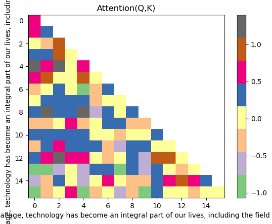
这段代码实现了 Transformer 多头注意力机制中注意力分数（Attention Score）的计算，并通过热图可视化展示了不同位置之间的注意力关联强度，是理解注意力机制如何 “关注” 序列中不同元素

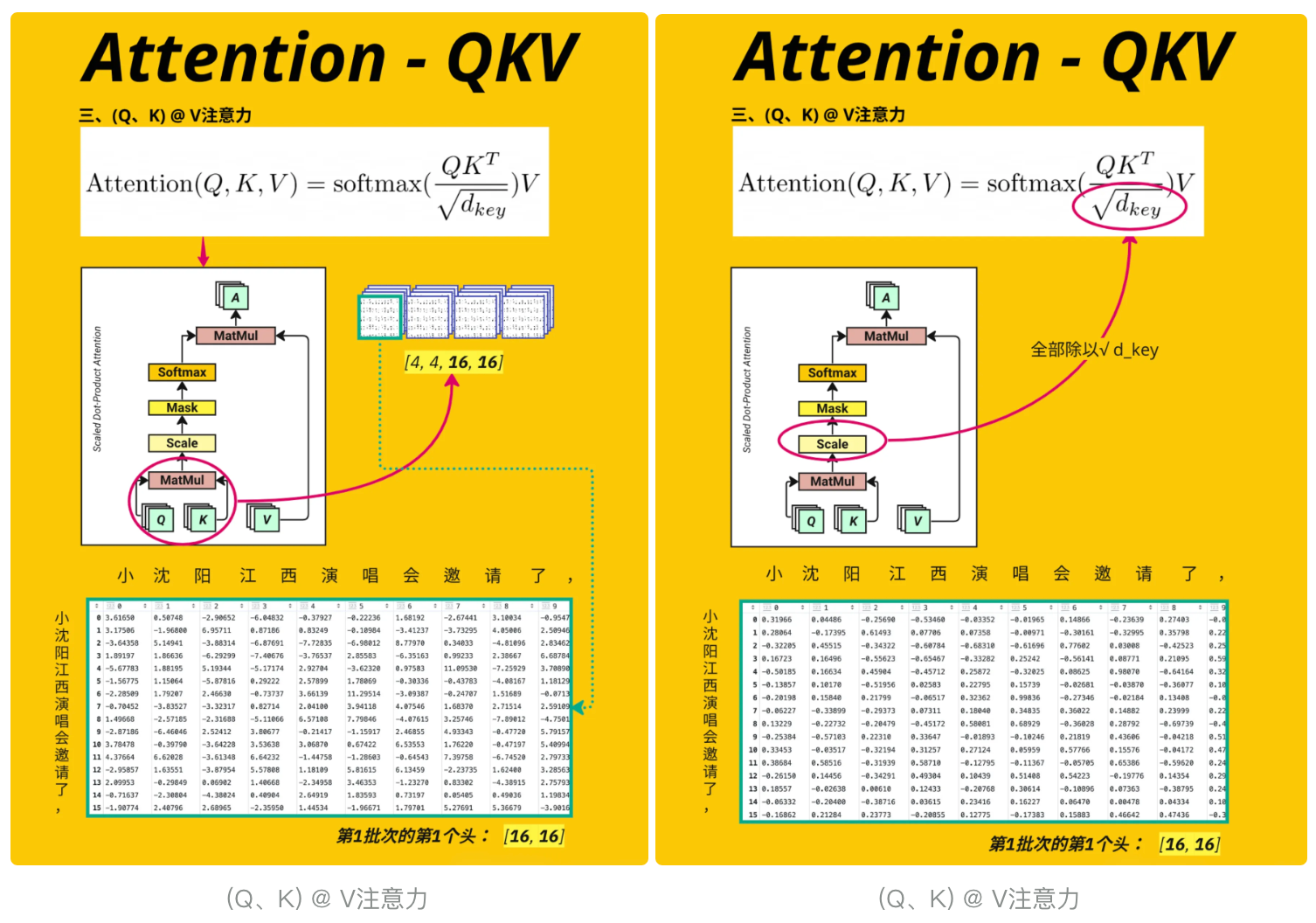
• K.transpose(-2, -1)：对 Key 进行转置，交换最后两个维度（-2和-1表示倒数第二和倒数第一维）
• torch.matmul(Q, K.transpose(-2, -1))：Q 与转置后的 K 进行矩阵乘法，计算 “查询 - 键” 的相似度（内积）
• / math.sqrt(d_model // num_heads)：对分数进行 “缩放”（Scaling）
• 见图 (Q、K) @ V注意力

# Calculate the attention scoreattention_score = torch.matmul(Q, K.transpose(-2, -1)) / math.sqrt(d_model // num_heads) # [4, 4, 16, 16]# Illustration onlyplt.imshow(attention_score[1, 1].detach().cpu().numpy(), \"Accent\", aspect=\"auto\")plt.title(\"Attention(Q @ K)\") #plot attention in the first head of the first batchplt.xlabel(encoding.decode(x_batch[0].tolist()))plt.ylabel(encoding.decode(x_batch[0].tolist()))plt.colorbar()pd.DataFrame(attention_score[0][0].detach().cpu().numpy())

3.4.5、掩码

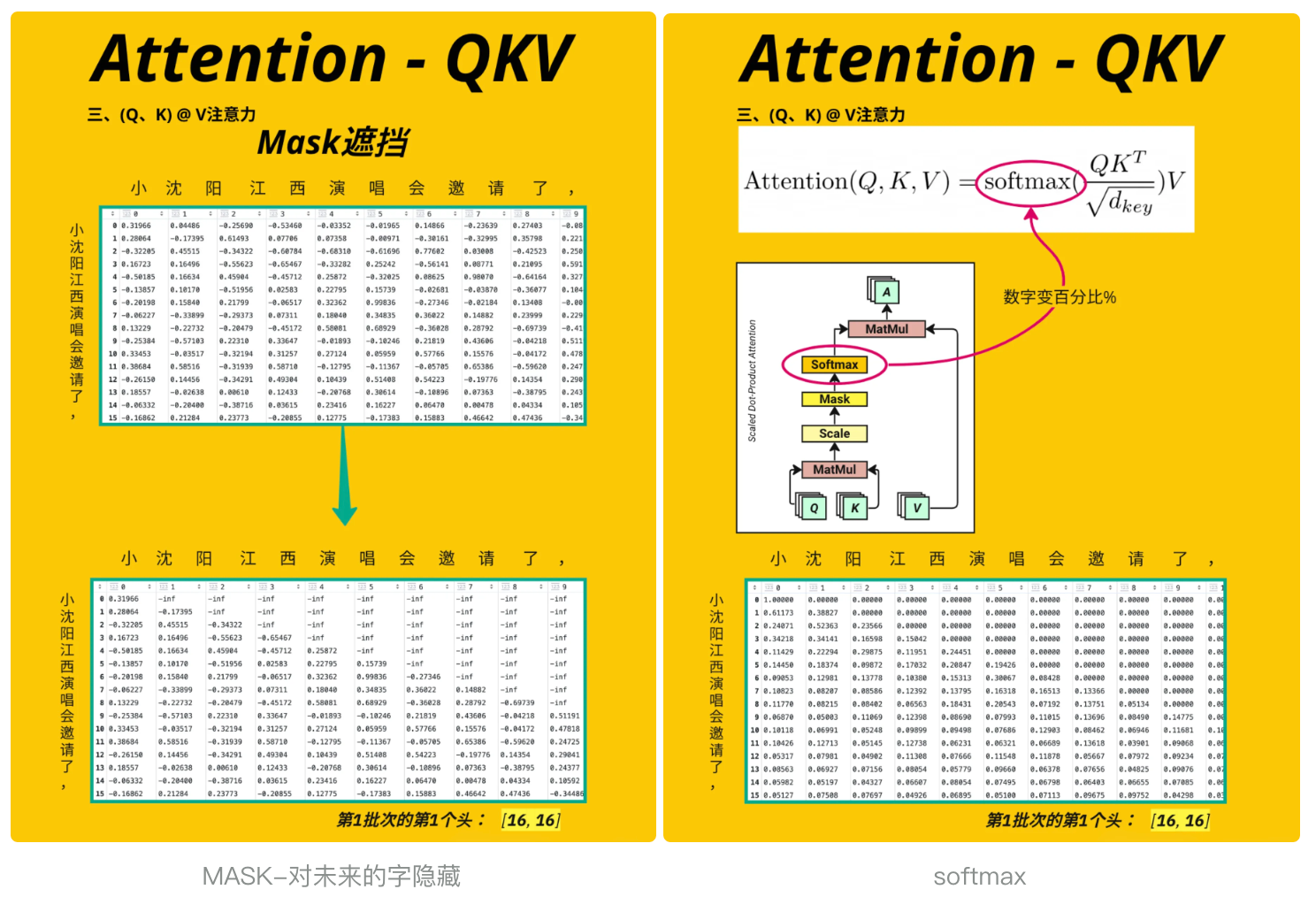
这段代码实现了 Transformer 模型中掩码（Mask）机制的核心操作 —— 通过掩盖 “未来位置” 的注意力分数，确保模型在处理序列时只能 “看到” 当前及之前的位置（无法预知未来信息）

• torch.ones(attention_score.shape[-2:])：生成一个形状为[context_length, context_length]（示例中[16,16]）的全 1 矩阵。shape[-2:]表示取注意力分数最后两个维度（序列长度 × 序列长度）
• torch.triu(..., diagonal=1)：将全 1 矩阵转换为上三角矩阵（主对角线以上的元素为 1，主对角线及以下为 0）。diagonal=1表示从主对角线的上一行开始为 1
• .to(device).bool()：将掩码矩阵移动到与注意力分数相同的设备（GPU/CPU），并转换为布尔类型（True/False），其中True对应需要掩盖的位置。
• masked_fill(..., float(\'-inf\'))：将注意力分数中掩码为True的位置（即未来位置）填充为负无穷。这样做的原因是：后续会对注意力分数应用softmax，而softmax(-inf) = 0，即这些位置的注意力权重会被归零，模型无法 “关注” 它们。

# 见图 MASK-对未来的字隐藏# Apply Mask to attention scoresattention_score = attention_score.masked_fill(torch.triu(torch.ones(attention_score.shape[-2:]).to(device), diagonal=1).bool(), float(\'-inf\'))#[4, 4, 16, 16] [batch_size, num_heads, context_length, context_length]# 可视化第二个样本（索引1）、第二个注意力头（索引1）的掩码后分数plt.imshow(attention_score[1, 1].detach().cpu().numpy(), \"Accent\", aspect=\"auto\")plt.title(\"Attention(Q,K) with Mask\") # 标题：带掩码的注意力分数plt.xlabel(encoding.decode(x_batch[0].tolist())) # x轴：被关注的位置（token）plt.ylabel(encoding.decode(x_batch[0].tolist())) # y轴：关注者的位置（token）plt.colorbar()pd.DataFrame(attention_score[0][0].detach().cpu().numpy())

与之前的可视化相比，此时热图的右上角区域（未来位置）会显示为负无穷（在热图中通常表现为最深的颜色或特殊值），直观展示了 “未来位置被掩盖” 的效果

3.4.6、Softmax

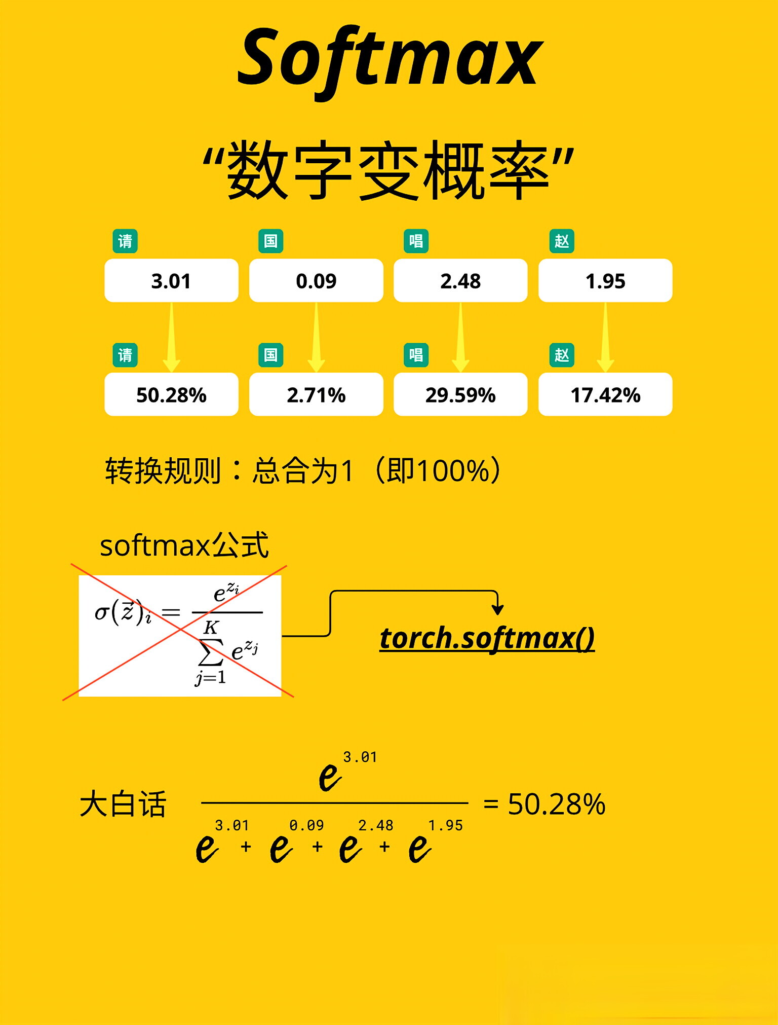
这段代码的作用是对经过掩码处理的注意力分数进行 Softmax 归一化，将其转换为符合概率分布的 “注意力权重”（Attention Weights）,见 图softmax

• torch.softmax(..., dim=-1)：
  • dim=-1表示在张量的最后一个维度上应用 Softmax 函数（这里最后一个维度是 “被关注的位置” 维度，即context_length）。
  • 对每个位置i（纵轴），Softmax 会将其对应的所有位置j（横轴）的注意力分数转换为 0~1 之间的权重，且所有j的权重之和为 1

# Softmax the attention scoreattention_score = torch.softmax(attention_score, dim=-1) #[4, 4, 16, 16] [batch_size, num_heads, context_length, context_length]pd.DataFrame(attention_score[0][0].detach().cpu().numpy())

3.4.7、与 V 相乘

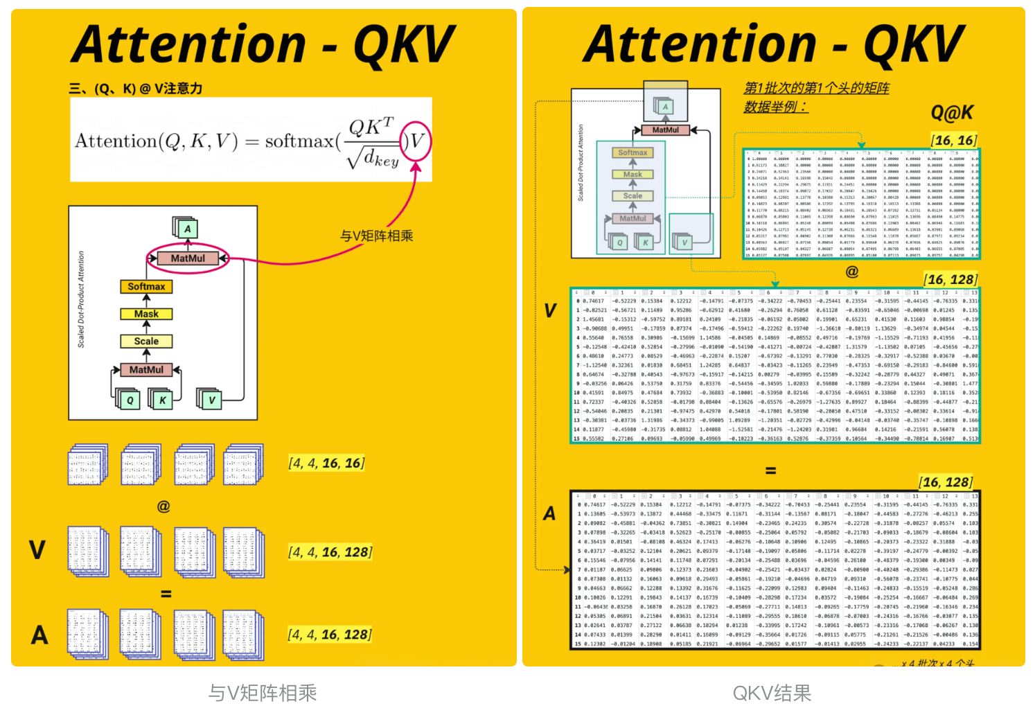
这段代码实现了多头注意力机制中将注意力权重与 Value 向量相乘的核心步骤, 见 图与V矩阵相乘

• attention_score（注意力权重）：最后两维是 [context_length, context_length]（16×16），表示 “每个位置对所有位置的关注权重”。
• V（Value 向量）：最后两维是 [context_length, head_size]（16×16），表示 “每个位置的 Value 特征向量”。

# Calculate the V attention outputprint(attention_score.shape) #[4, 4, 16, 16] [batch_size, num_heads, context_length, context_length]print(V.shape) #[4, 4, 16, 16] [batch_size, num_heads, context_length, head_size]A = torch.matmul(attention_score, V) # [4, 4, 16, 16] [batch_size, num_heads, context_length, head_size]print(A.shape)

torch.Size([4, 4, 16, 16])torch.Size([4, 4, 16, 16])torch.Size([4, 4, 16, 16])

3.4.8、多头合并

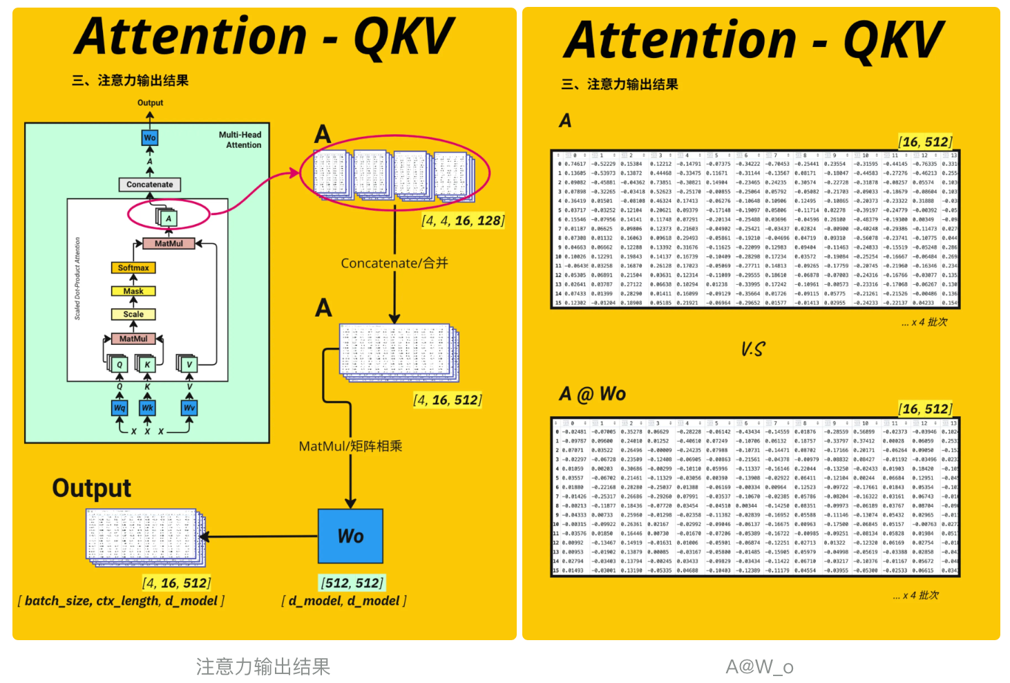
这段代码实现了多头注意力机制中将多个注意力头的输出拼接（Concatenate）并恢复原始维度的操作，是多头注意力从 “分头计算” 到 “合并结果”, 见 图注意力输出结果

• transpose(1, 2) 交换 1 维和 2 维后，新形状为 [batch_size, context_length, num_heads, head_size]
• reshape 操作的核心是将 “注意力头” 和 “头维度” 合并为原始的d_model维度：
  • 原后两维为 [num_heads, head_size]（4×16），两者相乘恰好等于 d_model（64）。
  • -1 表示自动计算该维度（这里对应context_length，保持 16 不变）。

# Concatenate the attention outputA = A.transpose(1, 2) # [4, 16, 4, 16] [batch_size, context_length, num_heads, head_size]A = A.reshape(batch_size, -1, d_model) # [4, 16, 64] [batch_size, context_length, d_model]A.shape

torch.Size([4, 16, 64])

这里对QKV、A的结果做一下说明

• Q@K的结果 : 每一个token对应其他token的权重(百分比)
• V : 原始词向量token (随机初始化)
• A: 样本文字中每个字对应样本其他所有文字再128个维度下的关注度权重总和 --> 训练过程中会不断发生变化, 改变初始值token

3.4.9、输出投影

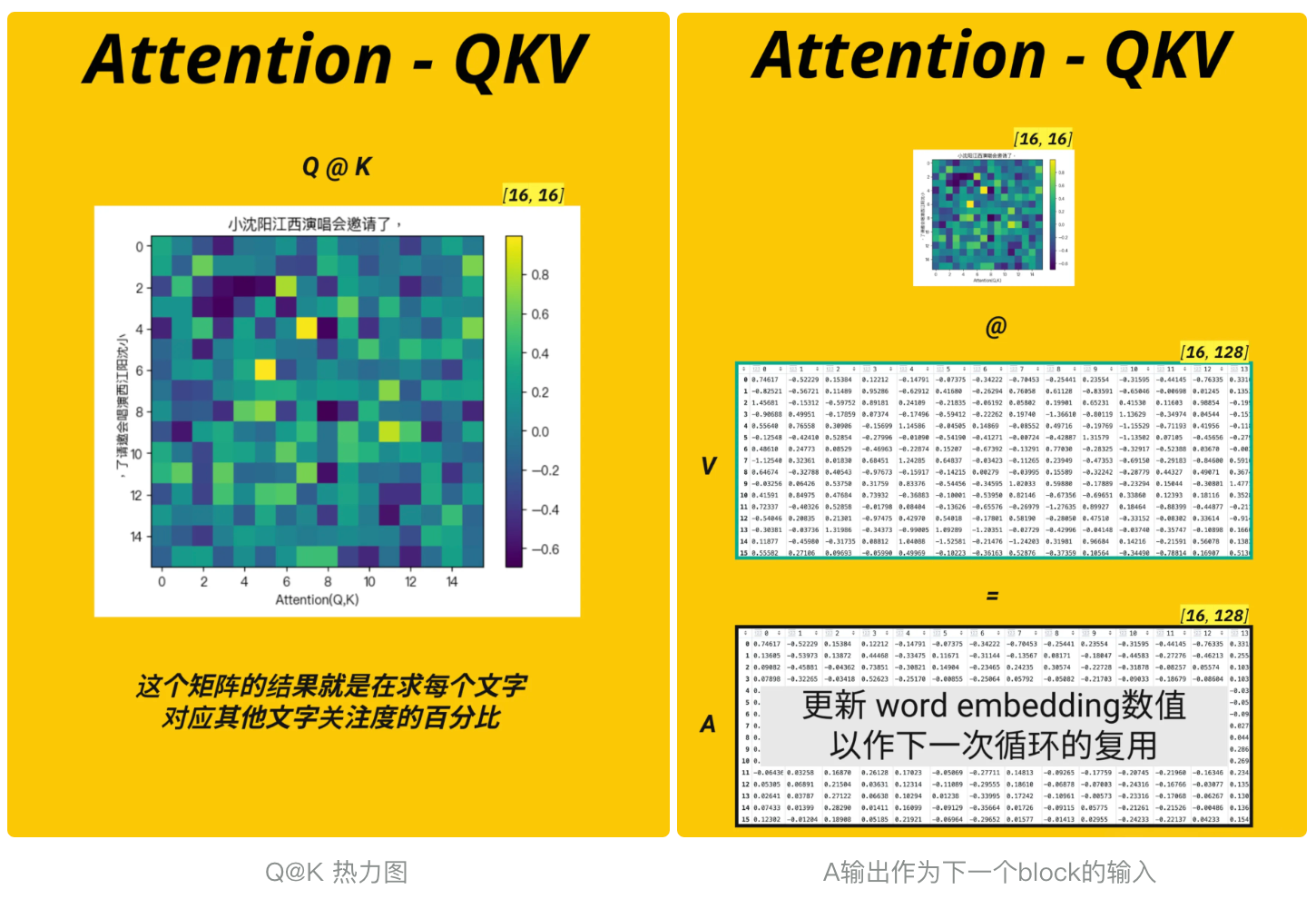
通过一个输出权重矩阵对合并后的多头注意力结果进行线性变换，得到最终的注意力输出，完成整个多头注意力的计算流程, 见 图A@W_o , A输出作为下一个block的输入

# Define the output weight matrixWo = nn.Linear(d_model, d_model).to(device)output = Wo(A) # [4, 16, 64] [batch_size, context_length, d_model]print(output.shape)pd.DataFrame(output[0].detach().cpu().numpy())

torch.Size([4, 16, 64])

至此整个多头注意力的流程至此完成：从输入生成 Q/K/V → 多头切分 → 计算注意力分数 → 掩码 → Softmax → 与 V 相乘 → 多头合并 → 输出投影，最终得到能够捕捉序列关联信息的特征表示

架构图红色方块里多头注意力机制的核心作用我在再总结下 :

• 将预设初始化的词嵌入向量token数值调整准确
• 将线性变换的权重调准确 (W_q, W_k, W_v, W_o)

3.4.10、残差连接和层归一化

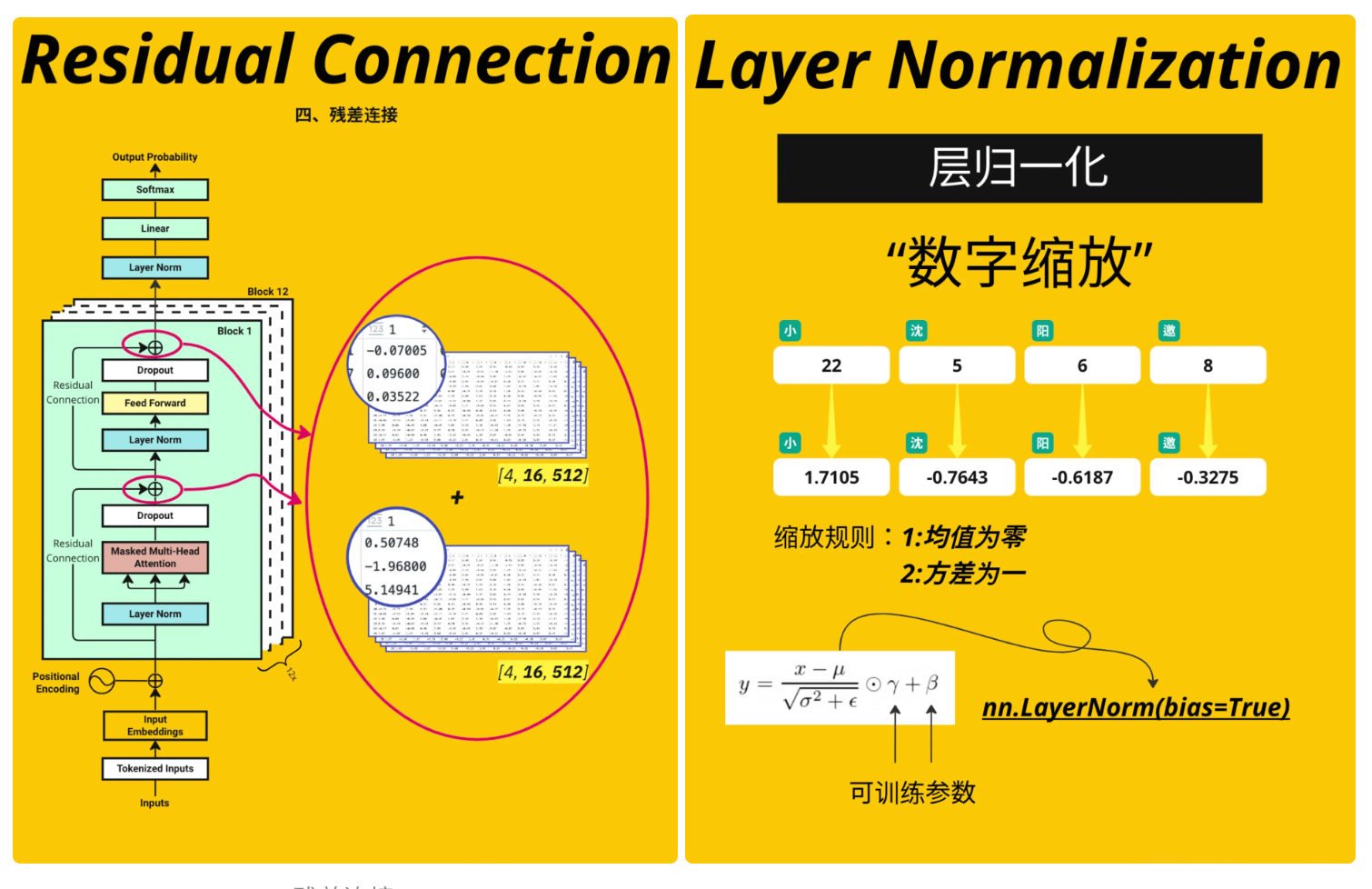
残差连接为了防止梯度爆炸和梯度消失, 有残差连接就是在相对小的范围内寻找最佳位置

# Add residual connectionoutput = output + X

# Add Layer Normalizationlayer_norm = nn.LayerNorm(d_model).to(device)output_layernorm = layer_norm(output).to(device)

3.4.11、前馈网络(Feed Forward Network)

前馈网络的作用是对序列中每个位置的特征进行独立的非线性变换（不涉及位置间的交互，与多头注意力的 “全局关联” 互补）。通过 “升维→非线性激活→降维” 的流程，模型能够捕捉更精细的局部特征，与多头注意力捕捉的全局关联信息结合，形成更全面的特征表示

• nn.Linear(d_model, d_model * 4)：定义一个线性层，将输入维度从d_model（模型特征维度，如 64）提升到d_model * 4（如 256）
• 输入output_layernorm：通常是经过 “多头注意力 + 残差连接 + 层归一化” 后的输出，形状为[batch_size, context_length, d_model]
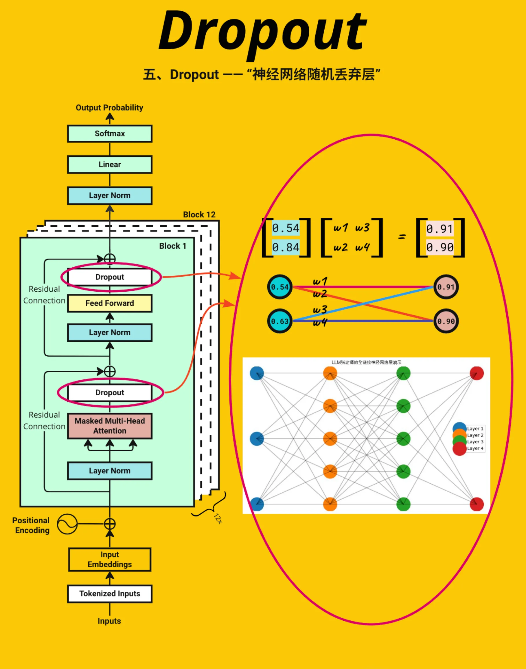
• 对升维后的特征应用ReLU 激活函数（ReLU(x) = max(0, x)），将负数特征置为 0，保留正数特征
• nn.Linear(d_model * 4, d_model)：定义第二个线性层，将中间维度（d_model * 4）还原回原始的d_model维度
• 应用dropout 正则化：在训练时，以概率p（如 0.1）随机将部分特征值置为 0，减少神经元之间的 “共适应”（过度依赖彼此），防止模型过拟合

# Define Feed Forward Networkoutput = nn.Linear(d_model, d_model * 4).to(device)(output_layernorm)output = nn.ReLU()(output)output = nn.Linear(d_model * 4, d_model).to(device)(output)output = torch.dropout(output, p=dropout, train=True)

这段代码实现了 Transformer 模型中单个 “Transformer 块（Block）” 的最终处理步骤—— 通过残差连接（Residual Connection）和层归一化（Layer Normalization）稳定特征分布，是构成深层 Transformer 模型的关键收尾操作

# Add residual connection & layerNorm (last time in a Transformer block)output = output + output_layernorm# Add Layer Normalizationlayer_norm = nn.LayerNorm(d_model).to(device)output = layer_norm(output)print(output.shape)

torch.Size([4, 16, 64])

前面的代码已经完整实现了一个 Transformer 块（Transformer Block）的逻辑，而实际的 Transformer 模型需要将这个块重复堆叠num_layers次（通常是 6、12、24 等），只是当前为了演示单个块的工作原理而省略了循环过程,后续可以自己写代码实践,提升模型预测准确率

4、单词预测

通过一个最终的线性层，将 Transformer 块输出的抽象特征向量，映射为每个 token 的 “原始预测分数（Logits）”，为后续计算概率或损失做准备

# Apply the final linear layer to get the logitslogits = nn.Linear(d_model, max_token_value+1).to(device)(output)pd.DataFrame(logits[0].detach().cpu().numpy())

这段代码的作用是将模型输出的原始预测分数（Logits）转换为符合概率分布的预测概率，让模型的预测结果更具可解释性，是从 “分数” 到 “概率” 的关键转换

probabilities = torch.softmax(logits, dim=-1)pd.DataFrame(probabilities[0].detach().cpu().numpy())

从模型的预测结果中提取第一个位置的最可能 token，并将其解码为原始的英文单词

# Let\'s see the predicted token and it\'s original English wordpredicted_index = torch.argmax(logits[0,0]).item()encoding.decode([predicted_index])

\'Catholics\'

看一下原始输入的句子

encoding.decode(x_batch[0].tolist())

\' digital age, technology has become an integral part of our lives, including the field\'

预测不准确的原因：Transformer 这类深度模型需要通过多轮训练（通常是成千上万次迭代）来调整海量参数（权重矩阵如 Wq、Wk、Wo 等），仅一次训练循环几乎无法让模型学到有意义的模式，预测结果自然可能偏离正确答案

以上就是一个最简单的Transformer实现代码

接下来,同学们可以自己再自由发挥了,为后面学习其他大语言模型打下基础

5、参考资料

《Attention is all you need》论文解读及Transformer架构详细介绍_哔哩哔哩_bilibiliPPT、论文笔记版github地址：https://github.com/huangyf2013320506/bilibili_repository, 视频播放量 313585、弹幕量 670、点赞数 21288、投硬币枚数 14886、收藏人数 39468、转发人数 3500, 视频作者 堂吉诃德拉曼查的英豪, 作者简介 是活的不是AI，相关视频：Transformer论文逐段精读【论文精读】，【高清中英】2025年吴恩达详细讲解Transformer工作原理，这次总能听懂了吧！ --人工智能/Trasnformer，【Transformer】最强动画讲解！目前B站最全最详细的Transformer教程，2025最新版！从理论到实战，通俗易懂解释原理，草履虫都学的会！，一小时从函数到Transformer！一路大白话彻底理解AI原理，【B站最新】吴恩达详细讲解Transformer工作原理，小白教程，全程干货无尿点，学完你就是AGI的大佬！（附课件+代码），【官方双语】直观解释注意力机制，Transformer的核心 | 【深度学习第6章】，【机器学习】【白板推导系列】【合集 1～33】，吴恩达同步最新AI课，第86讲：Claude Code-高智能的编程助手-A Highly Agentic Coding Assistant，【B站强推】浙大团队大模型公开课，2025最新浙大内部版大模型课程，大模型原理与技术教程，从入门到进阶，全程干货讲解，通俗易懂！1-1 基于统计的语言模型，彻底解读《Attention is All You Need》及Transformer架构https://www.bilibili.com/video/BV1xoJwzDESD/?share_source=copy_web&vd_source=091304ed9cc53ea1b8b1c52f53d5e65e

You will be redirected shortlyhttps://waylandzhang.github.io