数学建模常用30个算法——Python代码(二)_python 数学建模
数学建模常用算法
- 3. 优化算法
-
- 粒子群优化(PSO)模型
- 模拟退火(SA)模型
- 遗传算法(GA)
- 线性规划(LP)模型
- 非线性规划(NLP)模型
- 二次规划(QP)模型
- 4. 综合评价方法
-
- TOPSIS综合评价模型
- 层次分析法(AHP)
- 模糊综合评价模型
- 多目标模糊综合评价模型
3. 优化算法
粒子群优化(PSO)模型
模拟鸟群觅食行为,通过个体和群体最优解迭代搜索最优解,适用于连续优化问题。
import numpy as npimport matplotlib.pyplot as pltfrom mpl_toolkits.mplot3d import Axes3Ddef fit_fun(x): # 适应函数 return sum(100.0 * (x[0][1:] - x[0][:-1] ** 2.0) ** 2.0 + (1 - x[0][:-1]) ** 2.0)class Particle: # 初始化 def __init__(self, x_max, max_vel, dim): self.__pos = np.random.uniform(-x_max, x_max, (1, dim)) # 粒子的位置 self.__vel = np.random.uniform(-max_vel, max_vel, (1, dim)) # 粒子的速度 self.__bestPos = np.zeros((1, dim)) # 粒子最好的位置 self.__fitnessValue = fit_fun(self.__pos) # 适应度函数值 def set_pos(self, value): self.__pos = value def get_pos(self): return self.__pos def set_best_pos(self, value): self.__bestPos = value def get_best_pos(self): return self.__bestPos def set_vel(self, value): self.__vel = value def get_vel(self): return self.__vel def set_fitness_value(self, value): self.__fitnessValue = value def get_fitness_value(self): return self.__fitnessValueclass PSO: def __init__(self, dim, size, iter_num, x_max, max_vel, tol, best_fitness_value=float(\'Inf\'), C1=2, C2=2, W=1): self.C1 = C1 self.C2 = C2 self.W = W self.dim = dim # 粒子的维度 self.size = size # 粒子个数 self.iter_num = iter_num # 迭代次数 self.x_max = x_max self.max_vel = max_vel # 粒子最大速度 self.tol = tol # 截至条件 self.best_fitness_value = best_fitness_value self.best_position = np.zeros((1, dim)) # 种群最优位置 self.fitness_val_list = [] # 每次迭代最优适应值 # 对种群进行初始化 self.Particle_list = [Particle(self.x_max, self.max_vel, self.dim) for i in range(self.size)] def set_bestFitnessValue(self, value): self.best_fitness_value = value def get_bestFitnessValue(self): return self.best_fitness_value def set_bestPosition(self, value): self.best_position = value def get_bestPosition(self): return self.best_position # 更新速度 def update_vel(self, part): vel_value = self.W * part.get_vel() + self.C1 * np.random.rand() * (part.get_best_pos() - part.get_pos()) \\ + self.C2 * np.random.rand() * (self.get_bestPosition() - part.get_pos()) vel_value[vel_value > self.max_vel] = self.max_vel vel_value[vel_value < -self.max_vel] = -self.max_vel part.set_vel(vel_value) # 更新位置 def update_pos(self, part): pos_value = part.get_pos() + part.get_vel() part.set_pos(pos_value) value = fit_fun(part.get_pos()) if value < part.get_fitness_value(): part.set_fitness_value(value) part.set_best_pos(pos_value) if value < self.get_bestFitnessValue(): self.set_bestFitnessValue(value) self.set_bestPosition(pos_value) def update_ndim(self): for i in range(self.iter_num): for part in self.Particle_list: self.update_vel(part) # 更新速度 self.update_pos(part) # 更新位置 self.fitness_val_list.append(self.get_bestFitnessValue()) # 每次迭代完把当前的最优适应度存到列表 print(\'第{}次最佳适应值为{}\'.format(i, self.get_bestFitnessValue())) if self.get_bestFitnessValue() < self.tol: break return self.fitness_val_list, self.get_bestPosition()if __name__ == \'__main__\': # test 香蕉函数 pso = PSO(4, 5, 10000, 30, 60, 1e-4, C1=2, C2=2, W=1) fit_var_list, best_pos = pso.update_ndim() print(\"最优位置:\" + str(best_pos)) print(\"最优解:\" + str(fit_var_list[-1])) plt.plot(range(len(fit_var_list)), fit_var_list, alpha=0.5)模拟退火(SA)模型
受冶金退火启发,通过概率性接受劣解避免局部最优,适用于组合优化问题。
#本功能实现最小值的求解#from matplotlib import pyplot as pltimport numpy as npimport randomimport mathplt.ion()#这里需要把matplotlib改为交互状态#初始值设定hi=3lo=-3alf=0.95T=100#目标函数def f(x): return 11*np.sin(x)+7*np.cos(5*x)##注意这里要是np.sin#可视化函数(开始清楚一次然后重复的画)def visual(x): plt.cla() plt.axis([lo-1,hi+1,-20,20]) m=np.arange(lo,hi,0.0001) plt.plot(m,f(m)) plt.plot(x,f(x),marker=\'o\',color=\'black\',markersize=\'4\') plt.title(\'temperature={}\'.format(T)) plt.pause(0.1)#如果不停啥都看不见#随机产生初始值def init(): return random.uniform(lo,hi)#新解的随机产生def new(x): x1=x+T*random.uniform(-1,1) if (x1<=hi)&(x1>=lo): return x1 elif x1<lo: rand=random.uniform(-1,1) return rand*lo+(1-rand)*x else: rand=random.uniform(-1,1) return rand*hi+(1-rand)*x#p函数def p(x,x1): return math.exp(-abs(f(x)-f(x1))/T)def main(): global x global T x=init() while T>0.0001: visual(x) for i in range(500): x1=new(x) if f(x1)<=f(x): x=x1 else: if random.random()<=p(x,x1): x=x1 else: continue T=T*alf print(\'最小值为:{}\'.format(f(x)))main()遗传算法(GA)
模拟自然选择过程,通过选择、交叉和变异操作优化解,适用于复杂非线性问题。
import numpy as npimport matplotlib.pyplot as pltfrom matplotlib import cmfrom mpl_toolkits.mplot3d import Axes3DDNA_SIZE = 24POP_SIZE = 200CROSSOVER_RATE = 0.8MUTATION_RATE = 0.005N_GENERATIONS = 50X_BOUND = [-3, 3]Y_BOUND = [-3, 3]def F(x, y):return 3*(1-x)**2*np.exp(-(x**2)-(y+1)**2)- 10*(x/5 - x**3 - y**5)*np.exp(-x**2-y**2)- 1/3**np.exp(-(x+1)**2 - y**2)def plot_3d(ax):X = np.linspace(*X_BOUND, 100)Y = np.linspace(*Y_BOUND, 100)X,Y = np.meshgrid(X, Y)Z = F(X, Y)ax.plot_surface(X,Y,Z,rstride=1,cstride=1,cmap=cm.coolwarm)ax.set_zlim(-10,10)ax.set_xlabel(\'x\')ax.set_ylabel(\'y\')ax.set_zlabel(\'z\')plt.pause(3)plt.show()def get_fitness(pop): x,y = translateDNA(pop)pred = F(x, y)return (pred - np.min(pred)) + 1e-3 #减去最小的适应度是为了防止适应度出现负数,通过这一步fitness的范围为[0, np.max(pred)-np.min(pred)],最后在加上一个很小的数防止出现为0的适应度def translateDNA(pop): #pop表示种群矩阵,一行表示一个二进制编码表示的DNA,矩阵的行数为种群数目x_pop = pop[:,1::2]#奇数列表示Xy_pop = pop[:,::2] #偶数列表示y#pop:(POP_SIZE,DNA_SIZE)*(DNA_SIZE,1) --> (POP_SIZE,1)x = x_pop.dot(2**np.arange(DNA_SIZE)[::-1])/float(2**DNA_SIZE-1)*(X_BOUND[1]-X_BOUND[0])+X_BOUND[0]y = y_pop.dot(2**np.arange(DNA_SIZE)[::-1])/float(2**DNA_SIZE-1)*(Y_BOUND[1]-Y_BOUND[0])+Y_BOUND[0]return x,ydef crossover_and_mutation(pop, CROSSOVER_RATE = 0.8):new_pop = []for father in pop:#遍历种群中的每一个个体,将该个体作为父亲child = father#孩子先得到父亲的全部基因(这里我把一串二进制串的那些0,1称为基因)if np.random.rand() < CROSSOVER_RATE:#产生子代时不是必然发生交叉,而是以一定的概率发生交叉mother = pop[np.random.randint(POP_SIZE)]#再种群中选择另一个个体,并将该个体作为母亲cross_points = np.random.randint(low=0, high=DNA_SIZE*2)#随机产生交叉的点child[cross_points:] = mother[cross_points:]#孩子得到位于交叉点后的母亲的基因mutation(child)#每个后代有一定的机率发生变异new_pop.append(child)return new_popdef mutation(child, MUTATION_RATE=0.003):if np.random.rand() < MUTATION_RATE: #以MUTATION_RATE的概率进行变异mutate_point = np.random.randint(0, DNA_SIZE)#随机产生一个实数,代表要变异基因的位置child[mutate_point] = child[mutate_point]^1 #将变异点的二进制为反转def select(pop, fitness): # nature selection wrt pop\'s fitness idx = np.random.choice(np.arange(POP_SIZE), size=POP_SIZE, replace=True, p=(fitness)/(fitness.sum()) ) return pop[idx]def print_info(pop):fitness = get_fitness(pop)max_fitness_index = np.argmax(fitness)print(\"max_fitness:\", fitness[max_fitness_index])x,y = translateDNA(pop)print(\"最优的基因型:\", pop[max_fitness_index])print(\"(x, y):\", (x[max_fitness_index], y[max_fitness_index]))if __name__ == \"__main__\":fig = plt.figure()ax = Axes3D(fig)plt.ion()#将画图模式改为交互模式,程序遇到plt.show不会暂停,而是继续执行plot_3d(ax)pop = np.random.randint(2, size=(POP_SIZE, DNA_SIZE*2)) #matrix (POP_SIZE, DNA_SIZE)for _ in range(N_GENERATIONS):#迭代N代x,y = translateDNA(pop)if \'sca\' in locals(): sca.remove()sca = ax.scatter(x, y, F(x,y), c=\'black\', marker=\'o\');plt.show();plt.pause(0.1)pop = np.array(crossover_and_mutation(pop, CROSSOVER_RATE))#F_values = F(translateDNA(pop)[0], translateDNA(pop)[1])#x, y --> Z matrixfitness = get_fitness(pop)pop = select(pop, fitness) #选择生成新的种群print_info(pop)plt.ioff()plot_3d(ax)线性规划(LP)模型
在约束条件下优化线性目标函数,广泛应用于资源分配、生产计划等。
标准形式为:min z=2X1+3X2+xs.tx1+4x2+2x3>=83x1+2x2>=6x1,x2,x3>=0上述线性规划问题Python代码import numpy as npfrom scipy.optimize import linprogc = np.array([2, 3, 1])A_up = np.array([[-1, -4, -2], [-3, -2, 0]])b_up = np.array([-8, -6])r = linprog(c, A_ub=A_up, b_ub=b_up, bounds=((0, None), (0, None), (0, None)))print(r)非线性规划(NLP)模型
目标函数或约束为非线性,需梯度下降、牛顿法等数值方法求解。
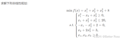
from scipy import optimize as optimport numpy as npfrom scipy.optimize import minimize# 目标函数def objective(x):return x[0] ** 2 + x[1] ** 2 + x[2] ** 2 + 8# 约束条件def constraint1(x):return x[0] ** 2 - x[1] + x[2] ** 2 # 不等约束def constraint2(x):return -(x[0] + x[1] ** 2 + x[2] ** 2 - 20) # 不等约束def constraint3(x):return -x[0] - x[1] ** 2 + 2def constraint4(x):return x[1] + 2 * x[2] ** 2 - 3 # 不等约束# 边界约束b = (0.0, None)bnds = (b, b, b)con1 = {\'type\': \'ineq\', \'fun\': constraint1}con2 = {\'type\': \'ineq\', \'fun\': constraint2}con3 = {\'type\': \'eq\', \'fun\': constraint3}con4 = {\'type\': \'eq\', \'fun\': constraint4}cons = ([con1, con2, con3, con4]) # 4个约束条件x0 = np.array([0, 0, 0])# 计算solution = minimize(objective, x0, method=\'SLSQP\', bounds=bnds, constraints=cons)x = solution.xprint(\'目标值: \' + str(objective(x)))print(\'答案为\')print(\'x1 = \' + str(x[0]))print(\'x2 = \' + str(x[1]))# ----------------------------------# 输出:# 目标值: 10.651091840572583# 答案为# x1 = 0.5521673412903173# x2 = 1.203259181851855二次规划(QP)模型
目标函数为二次型,约束为线性,常见于投资组合优化、控制理论。
工具包:Cvxopt python 凸优化包
函数原型:Cvxopt.solvers.qp(P,q,G,h,A,b)
P,q,G,h,A,b的含义参见上面的二次规划问题标准形式。
编程求解思路:
1.对于一个给定的二次规划问题,先转换为标准形式(参见数学基础中所讲的二次型二中形式转换)
2.对照标准形势,构建出矩阵P,q,G,h,A,b
3.调用result=Cvxopt.solvers.qp(P,q,G,h,A,b)求解
4.print(result)查看结果,其中result是一个字典,我们可直接获得其某个属性,e.g. print(result[‘x’])
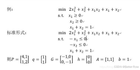
import pprintfrom cvxopt import matrix, solversP = matrix([[4.0,1.0],[1.0,2.0]])q = matrix([1.0,1.0])G = matrix([[-1.0,0.0],[0.0,-1.0]])h = matrix([0.0,0.0])A = matrix([1.0,1.0],(1,2))#原型为cvxopt.matrix(array,dims),等价于A = matrix([[1.0],[1.0]])b = matrix([1.0])result = solvers.qp(P,q,G,h,A,b) print(\'x\\n\',result[\'x\'])4. 综合评价方法
TOPSIS综合评价模型
通过计算与理想解和负理想解的相对接近度进行排序,适用于多指标决策分析。
import numpy as np # 导入numpy包并将其命名为np##定义正向化的函数def positivization(x,type,i):# x:需要正向化处理的指标对应的原始向量# typ:指标类型(1:极小型,2:中间型,3:区间型)# i:正在处理的是原始矩阵的哪一列 if type == 1: #极小型 print(\"第\",i,\"列是极小型,正向化中...\") posit_x = x.max(0)-x print(\"第\",i,\"列极小型处理完成\") print(\"--------------------------分隔--------------------------\") return posit_x elif type == 2: #中间型 print(\"第\",i,\"列是中间型\") best = int(input(\"请输入最佳值:\")) m = (abs(x-best)).max() posit_x = 1-abs(x-best)/m print(\"第\",i,\"列中间型处理完成\") print(\"--------------------------分隔--------------------------\") return posit_x elif type == 3: #区间型 print(\"第\",i,\"列是区间型\") a,b = [int(l) for l in input(\"按顺序输入最佳区间的左右界,并用逗号隔开:\").split(\",\")] m = (np.append(a-x.min(),x.max()-b)).max() x_row = x.shape[0] #获取x的行数 posit_x = np.zeros((x_row,1),dtype=float) for r in range(x_row): if x[r] < a: posit_x[r] = 1-(a-x[r])/m elif x[r] > b: posit_x[r] = 1-(x[r]-b)/m else: posit_x[r] = 1 print(\"第\",i,\"列区间型处理完成\") print(\"--------------------------分隔--------------------------\") return posit_x.reshape(x_row)## 第一步:从外部导入数据#注:保证表格不包含除数字以外的内容x_mat = np.loadtxt(\'river.csv\', encoding=\'UTF-8-sig\', delimiter=\',\') # 推荐使用csv格式文件## 第二步:判断是否需要正向化n, m = x_mat.shapeprint(\"共有\", n, \"个评价对象\", m, \"个评价指标\")judge = int(input(\"指标是否需要正向化处理,需要请输入1,不需要则输入0:\"))if judge == 1: position = np.array([int(i) for i in input(\"请输入需要正向化处理的指标所在的列,例如第1、3、4列需要处理,则输入1,3,4\").split(\',\')]) position = position-1 typ = np.array([int(j) for j in input(\"请按照顺序输入这些列的指标类型(1:极小型,2:中间型,3:区间型)格式同上\").split(\',\')]) for k in range(position.shape[0]): x_mat[:, position[k]] = positivization(x_mat[:, position[k]], typ[k], position[k]) print(\"正向化后的矩阵:\", x_mat)## 第三步:对正向化后的矩阵进行标准化tep_x1 = (x_mat * x_mat).sum(axis=0) # 每个元素平方后按列相加tep_x2 = np.tile(tep_x1, (n, 1)) # 将矩阵tep_x1平铺n行Z = x_mat / ((tep_x2) ** 0.5) # Z为标准化矩阵print(\"标准化后的矩阵为:\", Z)## 第四步:计算与最大值和最小值的距离,并算出得分tep_max = Z.max(0) # 得到Z中每列的最大值tep_min = Z.min(0) # 每列的最小值tep_a = Z - np.tile(tep_max, (n, 1)) # 将tep_max向下平铺n行,并与Z中的每个对应元素做差tep_i = Z - np.tile(tep_min, (n, 1)) # 将tep_max向下平铺n行,并与Z中的每个对应元素做差D_P = ((tep_a ** 2).sum(axis=1)) ** 0.5 # D+与最大值的距离向量D_N = ((tep_i ** 2).sum(axis=1)) ** 0.5S = D_N / (D_P + D_N) # 未归一化的得分std_S = S / S.sum(axis=0)sorted_S = np.sort(std_S, axis=0)print(std_S) # 打印标准化后的得分## std_S.to_csv(std_S.csv) 结果输出到std_S.csv文件层次分析法(AHP)
将复杂问题分层,通过成对比较矩阵计算权重,用于主观评价和决策。
import numpy as npclass AHP: \"\"\" 相关信息的传入和准备 \"\"\" def __init__(self, array): ## 记录矩阵相关信息 self.array = array ## 记录矩阵大小 self.n = array.shape[0] # 初始化RI值,用于一致性检验 self.RI_list = [0, 0, 0.52, 0.89, 1.12, 1.26, 1.36, 1.41, 1.46, 1.49, 1.52, 1.54, 1.56, 1.58, 1.59] # 矩阵的特征值和特征向量 self.eig_val, self.eig_vector = np.linalg.eig(self.array) # 矩阵的最大特征值 self.max_eig_val = np.max(self.eig_val) # 矩阵最大特征值对应的特征向量 self.max_eig_vector = self.eig_vector[:, np.argmax(self.eig_val)].real # 矩阵的一致性指标CI self.CI_val = (self.max_eig_val - self.n) / (self.n - 1) # 矩阵的一致性比例CR self.CR_val = self.CI_val / (self.RI_list[self.n - 1]) \"\"\" 一致性判断 \"\"\" def test_consist(self): # 打印矩阵的一致性指标CI和一致性比例CR print(\"判断矩阵的CI值为:\" + str(self.CI_val)) print(\"判断矩阵的CR值为:\" + str(self.CR_val)) # 进行一致性检验判断 if self.n == 2: # 当只有两个子因素的情况 print(\"仅包含两个子因素,不存在一致性问题\") else: if self.CR_val < 0.1: # CR值小于0.1,可以通过一致性检验 print(\"判断矩阵的CR值为\" + str(self.CR_val) + \",通过一致性检验\") return True else: # CR值大于0.1, 一致性检验不通过 print(\"判断矩阵的CR值为\" + str(self.CR_val) + \"未通过一致性检验\") return False \"\"\" 算术平均法求权重 \"\"\" def cal_weight_by_arithmetic_method(self): # 求矩阵的每列的和 col_sum = np.sum(self.array, axis=0) # 将判断矩阵按照列归一化 array_normed = self.array / col_sum # 计算权重向量 array_weight = np.sum(array_normed, axis=1) / self.n # 打印权重向量 print(\"算术平均法计算得到的权重向量为:\\n\", array_weight) # 返回权重向量的值 return array_weight \"\"\" 几何平均法求权重 \"\"\" def cal_weight__by_geometric_method(self): # 求矩阵的每列的积 col_product = np.product(self.array, axis=0) # 将得到的积向量的每个分量进行开n次方 array_power = np.power(col_product, 1 / self.n) # 将列向量归一化 array_weight = array_power / np.sum(array_power) # 打印权重向量 print(\"几何平均法计算得到的权重向量为:\\n\", array_weight) # 返回权重向量的值 return array_weight \"\"\" 特征值法求权重 \"\"\" def cal_weight__by_eigenvalue_method(self): # 将矩阵最大特征值对应的特征向量进行归一化处理就得到了权重 array_weight = self.max_eig_vector / np.sum(self.max_eig_vector) # 打印权重向量 print(\"特征值法计算得到的权重向量为:\\n\", array_weight) # 返回权重向量的值 return array_weightif __name__ == \"__main__\": # 给出判断矩阵 b = np.array([[1, 1 / 3, 1 / 8], [3, 1, 1 / 3], [8, 3, 1]]) # 算术平均法求权重 weight1 = AHP(b).cal_weight_by_arithmetic_method() # 几何平均法求权重 weight2 = AHP(b).cal_weight__by_geometric_method() # 特征值法求权重 weight3 = AHP(b).cal_weight__by_eigenvalue_method()模糊综合评价模型
结合模糊数学处理不确定性,适用于语言变量(如“高”“低”)的评价问题。
#模糊综合评价,计算模糊矩阵和指标权重import xlrddata=xlrd.open_workbook(r\'F:\\hufengling\\离线数据(更新)\\3.xlsx\') #读取研究数据# table1 = data.sheets()[0] #通过索引顺序获取# table1 = data.sheet_by_index(sheet_indx)) #通过索引顺序获取table2 = data.sheet_by_name(\'4day\')#通过名称获取# rows = table2.row_values(3) # 获取第四行内容cols1 = table2.col_values(0) # 获取第1列内容,评价指标1cols2 = table2.col_values(1) #评价指标2nrow=table2.nrows #获取总行数print(nrow)#分为四个等级,优、良、中、差,两个评价指标u1=0;u2=0;u3=0;u4=0 #用于计算每个等级下的个数,指标1t1=0;t2=0;t3=0;t4=0 #指标2for i in range(nrow): if cols1[i]<=0.018:u1+=1 elif cols1[i]<=0.028:u2+=1 elif cols1[i]<=0.038:u3+=1 else: u4+=1print(u1,u2,u3,u4)#每个等级下的概率pu1=u1/nrow;pu2=u2/nrow;pu3=u3/nrow;pu4=u4/nrowprint(pu1,pu2,pu3,pu4)du=[pu1,pu2,pu3,pu4]for i in range(nrow): if cols2[i]<=1:t1+=1 elif cols2[i]<=2:t2+=1 elif cols2[i]<=3:t3+=1 else: t4+=1print(t1,t2,t3,t4)pt1=t1/nrow;pt2=t2/nrow;pt3=t3/nrow;pt4=t4/nrowprint(pt1,pt2,pt3,pt4)dt=[pt1,pt2,pt3,pt4]#熵权法定义指标权重def weight(du,dt): import math k=-1/math.log(4) sumpu=0;sumpt=0;su=0;st=0 for i in range(4): if du[i]==0:su=0 else:su=du[i]*math.log(du[i]) sumpu+=su if dt[i]==0:st=0 else:st=dt[i]*math.log(dt[i]) sumpt+=st E1=k*sumpu;E2=k*sumpt E=E1+E2 w1=(1-E1)/(2-E);w2=(1-E2)/(2-E) return w1,w2def score(du,dt,w1,w2): eachS=[] for i in range(4): eachS.append(du[i]*w1+dt[i]*w2) return eachSw1,w2=weight(du,dt)S=score(du,dt,w1,w2) #S中含有四个值,分别对应四个等级,取其中最大的值对应的等级即是最后的评价结果print(w1,w2)print(S)多目标模糊综合评价模型
扩展模糊评价至多目标优化,兼顾多个冲突目标的权衡。
def frequency(matrix,p): \'\'\' 频数统计法确定权重 :param matrix: 因素矩阵 :param p: 分组数 :return: 权重向量 \'\'\' A = np.zeros((matrix.shape[0])) for i in range(0, matrix.shape[0]): ## 根据频率确定频数区间列表 row = list(matrix[i, :]) maximum = max(row) minimum = min(row) gap = (maximum - minimum) / p row.sort() group = [] item = minimum while(item < maximum): group.append([item, item + gap]) item = item + gap print(group) ## 初始化一个数据字典,便于记录频数 dataDict = {} for k in range(0, len(group)): dataDict[str(k)] = 0 ## 判断本行的每个元素在哪个区间内,并记录频数 for j in range(0, matrix.shape[1]): for k in range(0, len(group)): if(matrix[k, j] >= group[k][0]): dataDict[str(k)] = dataDict[str(k)] + 1 break print(dataDict) ## 取出最大频数对应的key,并以此为索引求组中值 index = int(max(dataDict,key=dataDict.get)) mid = (group[index][0] + group[index][1]) / 2 print(mid) A[i] = mid A = A / sum(A[:]) ## 归一化 return A