零基础-动手学深度学习-6.6 卷积神经网络(LeNet)
通过之前几节,我们学习了构建一个完整卷积神经网络的所需组件。
回想一下现在我们已经掌握了卷积层的处理方法,我们可以在图像中保留空间结构。 同时,用卷积层代替全连接层的另一个好处是:模型更简洁、所需的参数更少。
本节将介绍LeNet,它是最早发布的卷积神经网络之一,于80年代发明的为了识别手写数字,LeCun发表了第一篇通过反向传播成功训练卷积神经网络的研究!
6.6.1. LeNet
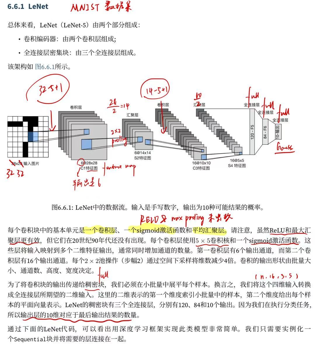
我这里改了一下28-32,实际上是32,但李沐老师修改成28然后加了填充边缘2,因此这里28卷积后维度不变。
import torchfrom torch import nnfrom d2l import torch as d2lnet = nn.Sequential( nn.Conv2d(1, 6, kernel_size=5, padding=2), nn.Sigmoid(), nn.AvgPool2d(kernel_size=2, stride=2), nn.Conv2d(6, 16, kernel_size=5), nn.Sigmoid(), nn.AvgPool2d(kernel_size=2, stride=2), nn.Flatten(), nn.Linear(16 * 5 * 5, 120), nn.Sigmoid(), nn.Linear(120, 84), nn.Sigmoid(), nn.Linear(84, 10))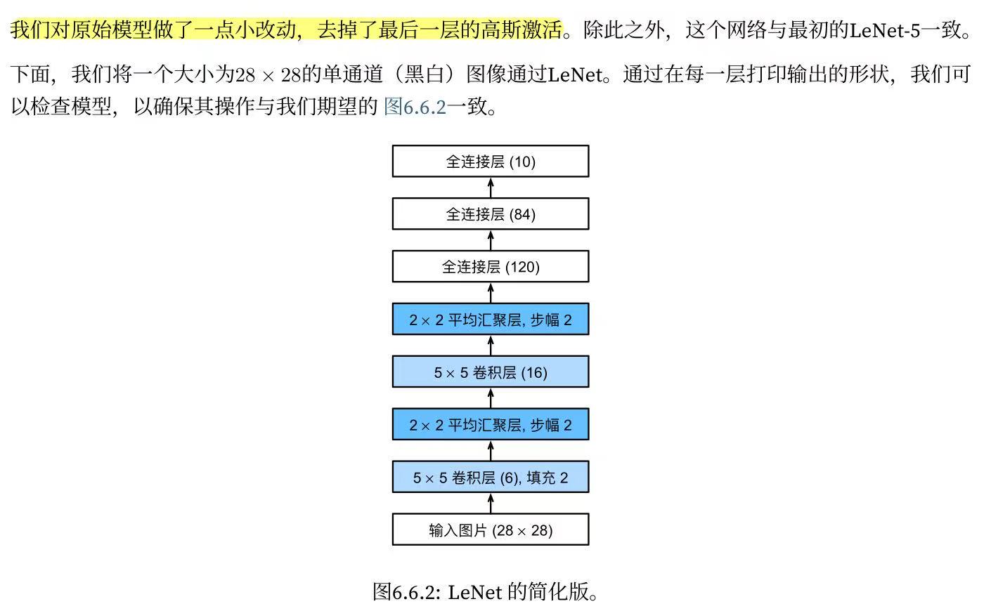
X = torch.rand(size=(1, 1, 28, 28), dtype=torch.float32)for layer in net: X = layer(X) print(layer.__class__.__name__,\'output shape: \\t\',X.shape)输出:Conv2d output shape: torch.Size([1, 6, 28, 28])Sigmoid output shape: torch.Size([1, 6, 28, 28])AvgPool2d output shape: torch.Size([1, 6, 14, 14])Conv2d output shape: torch.Size([1, 16, 10, 10])Sigmoid output shape: torch.Size([1, 16, 10, 10])AvgPool2d output shape: torch.Size([1, 16, 5, 5])Flatten output shape: torch.Size([1, 400])Linear output shape: torch.Size([1, 120])Sigmoid output shape: torch.Size([1, 120])Linear output shape: torch.Size([1, 84])Sigmoid output shape: torch.Size([1, 84])Linear output shape: torch.Size([1, 10])请注意,在整个卷积块中,与上一层相比,每一层特征的高度和宽度都减小了。 第一个卷积层使用2个像素的填充,来补偿5*5卷积核导致的特征减少。 相反,第二个卷积层没有填充,因此高度和宽度都减少了4个像素。 随着层叠的上升,通道的数量从输入时的1个,增加到第一个卷积层之后的6个,再到第二个卷积层之后的16个。 同时,每个汇聚层的高度和宽度都减半。最后,每个全连接层减少维数,最终输出一个维数与结果分类数相匹配的输出。
6.6.2. 模型训练
现在我们已经实现了LeNet,让我们看看LeNet在Fashion-MNIST数据集上的表现。
batch_size = 256train_iter, test_iter = d2l.load_data_fashion_mnist(batch_size=batch_size)虽然卷积神经网络的参数较少,但与深度的多层感知机相比,它们的计算成本仍然很高,因为每个参数都参与更多的乘法。 通过使用GPU,可以用它加快训练。
为了进行评估,我们需要对 3.6节中描述的evaluate_accuracy函数进行轻微的修改。 由于完整的数据集位于内存中,因此在模型使用GPU计算数据集之前,我们需要将其复制到显存中。
def evaluate_accuracy_gpu(net, data_iter, device=None): #@save \"\"\"使用GPU计算模型在数据集上的精度\"\"\" if isinstance(net, nn.Module): net.eval() # 设置为评估模式 if not device:#如果不是这个device就看一下你的设备在哪里 device = next(iter(net.parameters())).device # 正确预测的数量,总预测的数量 metric = d2l.Accumulator(2)#预设两个累加值 with torch.no_grad(): for X, y in data_iter: if isinstance(X, list): # BERT微调所需的(之后将介绍) X = [x.to(device) for x in X] else: X = X.to(device) y = y.to(device) metric.add(d2l.accuracy(net(X), y), y.numel()) return metric[0] / metric[1]为了使用GPU,我们还需要一点小改动。 与 3.6节中定义的train_epoch_ch3不同,在进行正向和反向传播之前,我们需要将每一小批量数据移动到我们指定的设备(例如GPU)上。
如下所示,训练函数train_ch6也类似于 3.6节中定义的train_ch3。 由于我们将实现多层神经网络,因此我们将主要使用高级API。 以下训练函数假定从高级API创建的模型作为输入,并进行相应的优化。 我们使用在 4.8.2.2节中介绍的Xavier随机初始化模型参数。 与全连接层一样,我们使用交叉熵损失函数和小批量随机梯度下降。
#@savedef train_ch6(net, train_iter, test_iter, num_epochs, lr, device): \"\"\"用GPU训练模型(在第六章定义)\"\"\" def init_weights(m):#初始化权重 if type(m) == nn.Linear or type(m) == nn.Conv2d:#如果是这几个层就进行xavier初始化 nn.init.xavier_uniform_(m.weight) net.apply(init_weights)#对网络的参数都初始化一下 print(\'training on\', device) net.to(device) optimizer = torch.optim.SGD(net.parameters(), lr=lr) loss = nn.CrossEntropyLoss() animator = d2l.Animator(xlabel=\'epoch\', xlim=[1, num_epochs], legend=[\'train loss\', \'train acc\', \'test acc\'])#动画效果 timer, num_batches = d2l.Timer(), len(train_iter) for epoch in range(num_epochs): # 训练损失之和,训练准确率之和,样本数 metric = d2l.Accumulator(3) net.train() for i, (X, y) in enumerate(train_iter): timer.start() optimizer.zero_grad() X, y = X.to(device), y.to(device)#移动参数 y_hat = net(X) l = loss(y_hat, y) l.backward() optimizer.step() with torch.no_grad(): metric.add(l * X.shape[0], d2l.accuracy(y_hat, y), X.shape[0]) timer.stop() train_l = metric[0] / metric[2] train_acc = metric[1] / metric[2] if (i + 1) % (num_batches // 5) == 0 or i == num_batches - 1: animator.add(epoch + (i + 1) / num_batches, (train_l, train_acc, None)) test_acc = evaluate_accuracy_gpu(net, test_iter)#下面都是打印信息 animator.add(epoch + 1, (None, None, test_acc)) print(f\'loss {train_l:.3f}, train acc {train_acc:.3f}, \' f\'test acc {test_acc:.3f}\') print(f\'{metric[2] * num_epochs / timer.sum():.1f} examples/sec \' f\'on {str(device)}\')现在,我们训练和评估LeNet-5模型
lr, num_epochs = 0.9, 10train_ch6(net, train_iter, test_iter, num_epochs, lr, d2l.try_gpu())输出:loss 0.469, train acc 0.823, test acc 0.77955296.6 examples/sec on cuda:0调参后结果还会更好!